1
$\begingroup$

I have 295 observations of two variables, of which here are a few:

 Date             Close price  
   1/04/14 0:00     478.72   
    2/04/14 0:00    437.51   
    3/04/14 0:00    447.08  
    4/04/14 0:00    448.88  
    5/04/14 0:00    464.83  
    6/04/14 0:00    460.70  
    7/04/14 0:00    446.22  
    8/04/14 0:00    450.46   
    9/04/14 0:00    440.20  
    10/04/14 0:00   360.84  
    11/04/14 0:00   420.06  
    12/04/14 0:00   420.66  
    13/04/14 0:00   414.95  
    14/04/14 0:00   457.63  
    15/04/14 0:00   520.12  
    16/04/14 0:00   529.16    

The first variable is the date plus time stamp "0:00" and the second variable is the price at that date. My whole data set spans 1/4/2014 till 20/1/2015 with daily observations.

I want to decompose this data into two components, trend and errors. I know stl is mainly for seasonal data, but I use the following code, setting the value of s.window to be large to negate the seasonality component.

btc.ts<-ts(btc.csv$Close.Price,frequency=12)
decomp<-stl(btc.ts,s.window=10000)
plot(decomp)

There are a few issues here, the frequency of my data is daily, and frequency = 12 is not correct, but my hopes are that I just want to extract the trend component of the stl and use the zoo package:

trend<-decomp$time.series[,"trend"]
td<-seq(as.Date("2014/4/1"),as.Date("2015/1/15"),"days")
trendz<-zoo(x=trend,order.by=td)

The reason for this is that the trend component found in stl looks the best out of all my approaches, as shown below:
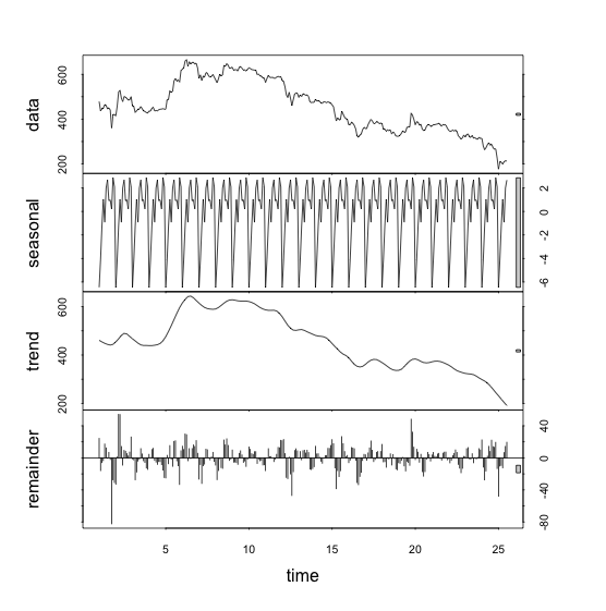
enter image description here

Now, what I want to do is fit a polynomial to model the trend, the issue I am having here is that I cannot use 'td' in the following command (natural splines):

trendz.fit<-lm(trendz~ns(td+I(td^2)+I(td^3)))

as td is a 'date' object. I just want to have something like : trend (t) = a + bt + c(t^2) + d(t^3)..

What can I do to achieve this? How does one usually treat regressions with one of the variables being time/date?

Any suggestions are appreciated, thanks

$\endgroup$
5
  • $\begingroup$ The plots make it clear a cubic will be a poor fit to these data. Higher-order polynomials will almost surely diverge wildly for predicting or retrodicting values. What, then, is your purpose in attempting a polynomial fit? $\endgroup$
    – whuber
    Commented Jan 26, 2015 at 17:38
  • $\begingroup$ @whuber admittedly I am new to this, do you have any suggestions for what would be a better way of going about this? $\endgroup$ Commented Jan 26, 2015 at 22:58
  • $\begingroup$ You haven't told us yet what you want to accomplish, so one could not in good conscience recommend anything at this point. What is the purpose of this exercise? What will you be doing with your fitted trend? $\endgroup$
    – whuber
    Commented Jan 26, 2015 at 23:08
  • $\begingroup$ @whuber I was hoping to replicate/extend the results of a paper I am reading where they fit a cubic polynomial to the trend, I've extended by expanding the number of observations, the paper : dept.econ.yorku.ca/~jasiakj/papers/ANCHR.pdf $\endgroup$ Commented Jan 26, 2015 at 23:17
  • 1
    $\begingroup$ As far as I can tell, the authors are uninterested in predicting the series itself. This paper focuses on analyzing the residuals from the trend in order to learn something about (and perhaps predict) bubbles in the detrended process. In effect, the trend is thrown away at the beginning without further analysis or comment. Cubic regression was likely chosen for its crudeness--it is a very heavy smooth--but also for having some flexibility to change its slope. If you want to emulate the paper, just dump the data into a polynomial fitting routine. Better, use a robust fitting routine. $\endgroup$
    – whuber
    Commented Jan 27, 2015 at 0:03

2 Answers 2

1
$\begingroup$

Regardless of which package you use, you would like to model a 'trend' as a polynomial. In your particular case, trend will be just what is left after seasonality and some 'random' noise were removed from the series. In order to model/check a trend, you proceed as any other regression. First, you need make your 'td' a vector of numbers i.e. $td.new=seq(1:length(td))$. For the $lm$ function to work it needs to be just plain integers. If there was a non-linear contribution, the $I(td.new^2)$ would just be significant as usual in linear regression...Hope this helps.

$\endgroup$
1
$\begingroup$

Consider the following,

> td
 [1] "2014-01-02" "2014-01-03" "2014-01-04" "2014-01-05" "2014-01-06"
 [6] "2014-01-07" "2014-01-08" "2014-01-09" "2014-01-10" "2014-01-11"

> class(td)
[1] "Date"

You can convert to a numeric variable by:

> td.num <- as.numeric(td - as.Date(1,origin="2014-01-01"))
> td.num
[1] 0 1 2 3 4 5 6 7 8 9

and this you can directly use in your regression.

$\endgroup$

Your Answer

By clicking “Post Your Answer”, you agree to our terms of service and acknowledge you have read our privacy policy.

Not the answer you're looking for? Browse other questions tagged or ask your own question.