How to simulate type I error and type II error

Question

Suppose $H_0: F_0$ and $H_1: F_1$, I want to simulate (lower bound of) the sum of type I($\alpha$) and type II($\beta$) error based on n observations. (Q:Am I posing the problem in the well-defined way?)

For simplicity, I am considering testing $H_0: \mu=0$ and $H_1: \mu=2$ for $F_0\sim N(0,1)$ and $F_1\sim N(2,1)$(Q: should $H_1$ be $\mu=2$ or just $\mu>0$?). For this setting, the minimum $\alpha+\beta$ occurs at the cut-off $\mu=1$. So maybe we can use this value to compare with test statistics($\bar{X}$)?

Then, how can I simulate the type I($\alpha$) and type II($\beta$) error? (I know the theoretical value of this sum is the area of the left tail of $F_1$ and right tail of $F_0$ separating from the cut-off point.)

Should I simulate say $n=100$ points, and 50 from $H_0$, and 50 from $H_1$(that is why I choose $H_1$ is $\mu=2$ rather than $\mu>0$, since I cannot simulate the later, right?). And count what is the misclassification rate, and that is the sum of $\alpha$ and $\beta$. Is this idea right? Am I asking a well-defined question?

Answer 1

First, a conventional way to write a test of hypothesis is:
$H_0: \mu=0$ and $H_1: \mu \ne 0$ or $H_1: \mu >0$ or $H_1: \mu <0$ based on the interest of the study.

Let's define Type I error:
Probability of rejecting null hypothesis when it is TRUE.

Type II error:
Probability of not rejecting null hypothesis when it is False.

Let's test type I error:

To observe the type I error of a test we need to generate/simulate data from the same distribution that follows null hypothesis. Notice the following R code:

n=10000 # testing 10,000 times
t1err=0
for (i in 1:n){
   x=rnorm(100, 0, 1)
   if (((t.test(x, mu=0))$p.value)<=0.05) (t1err=t1err+1) 
}
cat("Type I error rate in percentage is", (t1err/n)*100,"%")

It should give you about 5% error as Type I error.

Let's observe Type II error:
To test Type II error we have to generate/simulate data from another distribution than that followed by null hypothesis. Notice the following R code:

n=10000 # testing 10,000 times
t2err=0
for (i in 1:n){
   x=rnorm(100, 2, 1)
   if (((t.test(x, mu=0))$p.value)>0.05) (t2err=t2err+1) 
}
cat("Type II error rate in percentage is", (t2err/n)*100,"%")

You will see 0.0%. As the variance is really low. If you increase variance to 5, you will see about 2% error as Type II error.

Answer 2

Just to replicate this post dwelling on a different iteration of the same idea - in this case how quickly an unscrupulous researcher could generate throw-away pseudo-science with significant p values, I landed on this page, and learned from the accepted answer (+1).

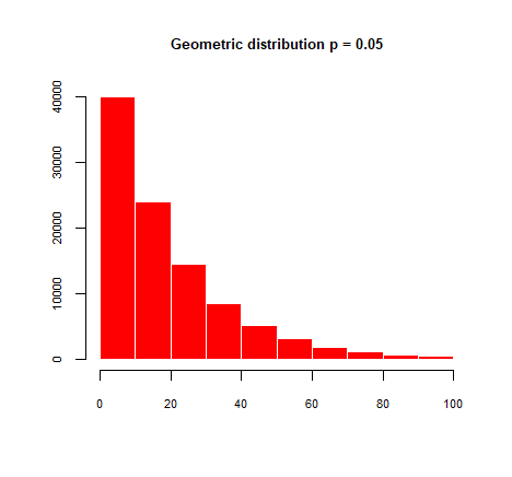
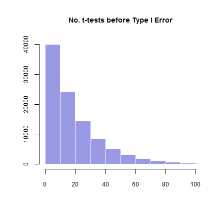
It turns out the mean is $20$ as predicted; the median is $14$; and the mode just $1.$ This is in keeping with the right skewed distribution on the histogram below.

Here is the code in R, and the results for mean, median and mode, which sounds like what you are asking in the follow-up comment:

set.seed(3141592)
firsthackingop <- 0  # Empty vec to collect number of studies before hitting the jackpot.
for(i in 1:1e5){     # The whole search for a sig p value will be done 100,000 times.
hackingwait <- 1     # The counting vector for every p-searching Safari.
  repeat{
  x=rnorm(100, 0, 1) # 100 draws from a norm dist as in @overwhelmed's answer.
  if(t.test(x, mu=0)$p.value > 0.05){hackingwait=hackingwait+1}else{break}
}
firsthackingop[i] <- hackingwait
}
mean(firsthackingop)
# [1] 20.17556
median(firsthackingop)
# [1] 14
Mode <- function(x) {
  ux <- unique(x)
  ux[which.max(tabulate(match(x, ux)))]
}
Mode(firsthackingop)
[1] 1
hist(firsthackingop, freq = T, main = "No. t-tests before Type I Error",
          xlim=c(0,100), col = rgb(.2,.2,.8,.5), border = F,
          cex.axis=.75, cex.main=.9, xlab="", ylab="")

Here is the histogram:

---

It is interesting to note that this is simply the geometric distribution with $p=0.05$ defined as The probability distribution of the number X of Bernoulli trials needed to get one success, which mean is $\frac{1}{p}=\frac{1}{0.05}=20;$ and with a mode of $1.$ The data generation in R is v = rgeom(1e5,0.05) + 1 and here is the plot:

> Mode(v)
[1] 1
> mean(v)
[1] 20.12817
> median(v)
[1] 14