Performing k-means clustering on a set of lines

Question

I have a set of lines (y = numbers between 1 and 100, x= discrete) that I am trying to cluster to group similarly-shaped profiles. I have found that the profiles seem to cluster the cleanest when only passing a smaller subset of the total x values to the k means function. Is this a valid approach? Can anyone point me in the direction of resources regarding clustering lines? Thanks in advance!

EDIT #2: My apologies for the confusion, I need to clarify. The data should be viewed similar to a timecourse.

EDIT #1:

For example, let d be a table containing 4 columns named 1:4, so that lines are plotted by row (eg the first line would contain 1, 24; 2,69; 3,91; 4,98)

1   2   3   4
24, 69  91  98
28, 76  98 108
21  63  88  95
10  36  69 101
75  85 104  94
70  68  90  82
39  67  91  89
35  68  90  90
52  68  63  47

The actual dataset has over 300 lines. Clustering using the data in all columns seems to give less "clean" results than by just clustering by columns a and d. I realize that "clean" is a very subjective term, but in this it seems that similar lines are grouped by only clustering by the points defining the end regions of the line.

In pseudocode:

full_cluster_list      = kmeans(d, 100 iterations, 5 centers)  
subsetted_cluster_list = kmeans(d[a,d], 100 iterations, 5 centers) 
  *#this seems to create tighter, cleaner clusters*

Answer 1

There are a couple of basic strategies to use with data like this. You can treat each point as a measurement on a different dimension, or you can fit models to each row / set of observations, and cluster the parameters of those models.

Here is an example with your data:

d    = read.table(text="1   2   3   4
                        ...  
                        52  68  63  47", header=T)
d.c  = as.data.frame(lapply(d, scale))
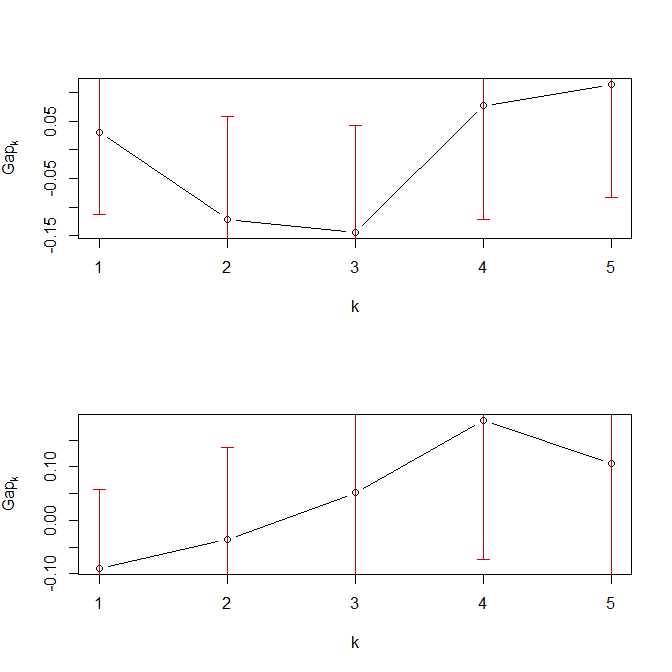
gap  = clusGap(d.c,          FUN=kmeans, K.max=5)
gap2 = clusGap(d.c[,c(1,4)], FUN=kmeans, K.max=5)
windows()
  layout(matrix(1:2, nrow=2))
  plot(gap)
  plot(gap2)

For your data, one cluster is probably the best result (and definitely better than two or three) when using all measurement occasions, but we'll pretend four is the way to go. Four is a clearer choice when using only the first and last occasions for this small (fake) dataset.

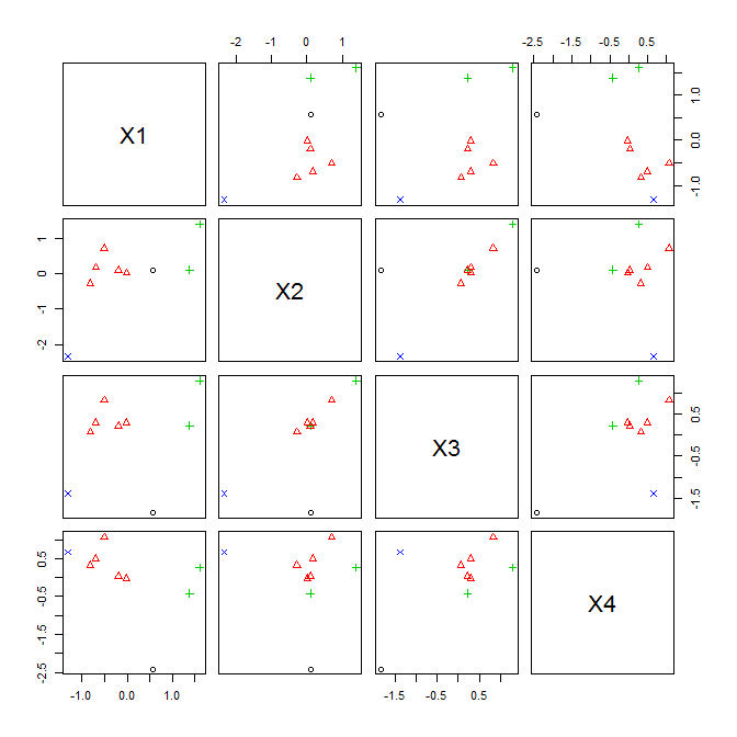
km4 = kmeans(d.c, 4);  km4  # uses all 4 measurement occasions
# K-means clustering with 4 clusters of sizes 1, 5, 2, 1
# 
# Cluster means:
#           X1         X2         X3          X4
# 1  0.5699003  0.1012253 -1.8486338 -2.41412585
# 2 -0.4469218  0.1467767  0.3441696  0.38017730
# 3  1.4922389  0.7465365  0.7581954 -0.07603546
# 4 -1.3197691 -2.3281815 -1.3886051  0.66531027
# 
# Clustering vector:
# [1] 2 2 2 4 3 3 2 2 1
# 
# Within cluster sum of squares by cluster:
# [1] 0.000000 2.067218 1.668397 0.000000
#  (between_SS / total_SS =  88.3 %)
# ...
windows()
  pairs(d.c, col=km4$cluster, pch=km4$cluster)

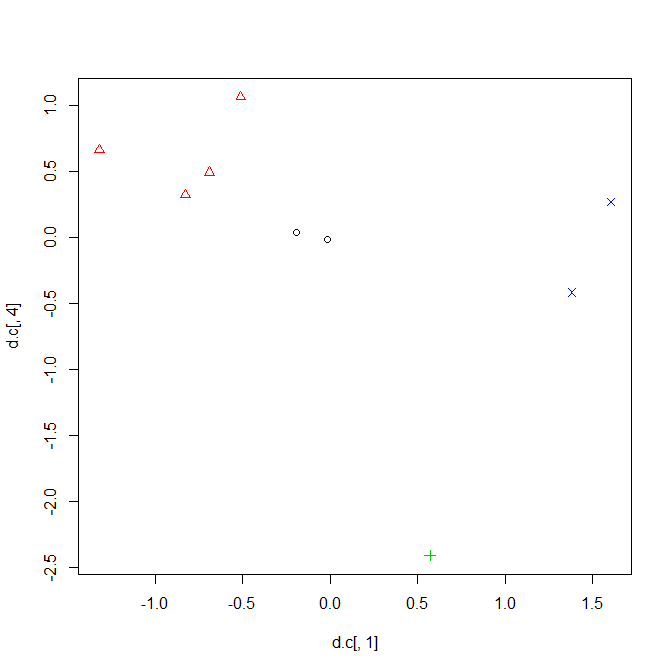
km2 = kmeans(d.c[,c(1,4)], 4);  km2  # uses only 2 measurement occasions
# K-means clustering with 4 clusters of sizes 2, 4, 1, 2
# 
# Cluster means:
#           X1           X4
# 1 -0.1049816  0.009504432
# 2 -0.8361037  0.636796976
# 3  0.5699003 -2.414125849
# 4  1.4922389 -0.076035460
# 
# Clustering vector:
# [1] 2 2 2 2 4 4 1 1 3
# 
# Within cluster sum of squares by cluster:
# [1] 0.01782035 0.66428113 0.00000000 0.25944999
#  (between_SS / total_SS =  94.1 %)
# ...
windows()
  plot(d.c[,1], d.c[,4], col=km2$cluster, pch=km2$cluster)

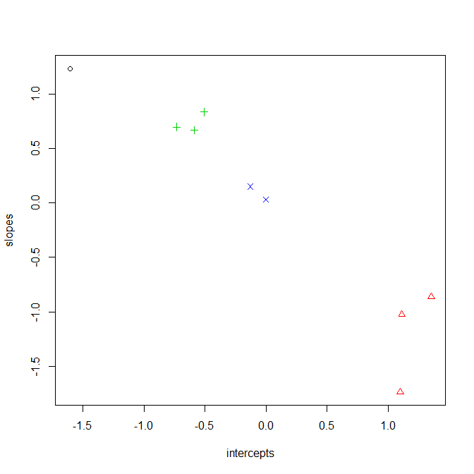
The alternative is to fit a model to each row and cluster the slopes and intercepts. If you are thinking of these as lines, this is probably the better approach. In addition, if you had an imbalanced dataset, this is probably the only meaningful way.

td = t(d)
cmat = matrix(NA, nrow=9, ncol=2)
for(j in 1:9){
  cmat[j,] = coef(lm(td[,j]~c(1:4)))
}

In this case, four clusters is the obvious solution (code and plot omitted).

ccmat = scale(cmat)
kmsi  = kmeans(ccmat, 4);  kmsi
# K-means clustering with 4 clusters of sizes 1, 3, 3, 2
# 
# Cluster means:
#          [,1]        [,2]
# 1 -1.60550223  1.23649307
# 2  1.18690594 -1.20811454
# 3 -0.60934903  0.73480121
# 4 -0.06358425  0.09172346
# 
# Clustering vector:
# [1] 3 3 3 1 2 2 4 4 2
# 
# Within cluster sum of squares by cluster:
# [1] 0.00000000 0.47392897 0.04091304 0.01511672
#  (between_SS / total_SS =  96.7 %)
# ...
windows()
  plot(ccmat[,1], ccmat[,2], xlab="intercepts", ylab="slopes", 
       col=kmsi$cluster, pch=kmsi$cluster)

Answer 2

Clustering will give good results when using significant data. What I mean is, if you have two random columns, you might not want to include them in your clustering algorithm because it would bring useless noise.

Clustering is actually all about feature selection (for a fixed clustering algorithm, e.g. K-means, EM...). You have to extract from you data what is most significant of the geometry of your problem. It is pretty hard to say, without any context if all your columns are significant or not. Conclusion is: there's no rule about getting clean result, you should first try to understand what represents most your problem and use it for clustering. Sometimes it means selecting few columns, sometimes take them all...