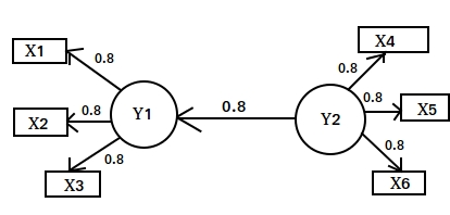
Assume we have the following linear path model:
Structural (inner) model:
$Y_{1} = \beta_{1}Y_{2}+\theta_{1}\delta$
Measurement (outer) model:
$X_{1} = \lambda_{1}*Y_{1}+\epsilon_{1}\delta$
$X_{2} = \lambda_{2}*Y_{1}+\epsilon_{2}\delta$
$X_{3} = \lambda_{3}*Y_{1}+\epsilon_{3}\delta$
$X_{4} = \lambda_{4}*Y_{2}+\epsilon_{4}\delta$
$X_{5} = \lambda_{5}*Y_{2}+\epsilon_{5}\delta$
$X_{6} = \lambda_{6}*Y_{2}+\epsilon_{6}\delta$
with: $X_{i}$ = manifest variables (indicators),
$Y_{i}$ = latent variables (constructs),
$\lambda_{i} = 0.8$,
$\beta_{1} = 0.8$,
$\epsilon_{i}$ = i.i.d.,
$\delta$ = some constant, which determines the strength of the error. Here delta is set to 0.6, because all correlations are 0.8 and a delta of 0.6 gives almost exact correlations of 0.8. So the purpose of delta is to get emprical correlations or at least pseudo empircal. I don't know if thats how its done, but it worked for this example.
The visual model looks as follows:

So I wrote some messy R Code to get the covariance matrix of the $X_{i}$:
library("MASS")

# set up covariance matrix of independent errors
sig <- matrix(0, 8, 8)
rownames(sig) <- c("y2", "e1", "e2", "e3", "e4", "e5", "e6", "d1")
colnames(sig) <- rownames(sig)
diag(sig) <- 1

# simulate random uncorrelated variables
rndm.vars <- mvrnorm(100, Sigma = sig, mu = c(0, 0, 0, 0, 0, 0, 0, 0), empirical = TRUE)

# split the simulated variables to the names in the equation for better readability
y2 <- rndm.vars[,1]
e1 <- rndm.vars[,2]
e2 <- rndm.vars[,3]
e3 <- rndm.vars[,4]
e4 <- rndm.vars[,5]
e5 <- rndm.vars[,6]
e6 <- rndm.vars[,7]
d1 <- rndm.vars[,8]

# set global delta
delta <- 0.6

# set path coefficients of the structural (inner) model
beta_1 <- 0.8

# linear equation of the inner model
y1 <- beta_1*y2+d1*delta

# set outer loadings (coefficients) of the measurement (outer) model
lam_i <- 0.8

## linear equations of the measurement (outer) model
# measurement model of y1
x1 <- y1*lam_i+e1*delta
x2 <- y1*lam_i+e2*delta
x3 <- y1*lam_i+e3*delta

# measurement model of y2
x4 <- y2*lam_i+e4*delta
x5 <- y2*lam_i+e5*delta
x6 <- y2*lam_i+e6*delta

# form a dataset from the manifest variables (indicators)
X <- cbind(x1, x2, x3, x4, x5, x6)
sim.data <- as.data.frame(X)

# get the covariance matrix of X
cor(X)

      x1    x2    x3    x4    x5    x6
x1 1.000 0.640 0.640 0.512 0.512 0.512
x2 0.640 1.000 0.640 0.512 0.512 0.512
x3 0.640 0.640 1.000 0.512 0.512 0.512
x4 0.512 0.512 0.512 1.000 0.640 0.640
x5 0.512 0.512 0.512 0.640 1.000 0.640
x6 0.512 0.512 0.512 0.640 0.640 1.000
So now lets do partial least squares structural equation modeling!
# Lets try sempls!!
library("semPLS")

# specify dataset
dataset <- as.data.frame(X)

## specify models
# measurement (outer) model
mm <- cbind(c("y1", "y1", "y1", "y2", "y2", "y2"),
                c("x1", "x2", "x3", "x4", "x5", "x6"))

# structural (inner) model
sm <- cbind(c("y2"), c("y1"))


# create plsm object
model <- plsm(dataset, sm, mm)

# estimate the model with the pls algorithm
estim.model <- sempls(model, dataset)

# show the results
estim.model

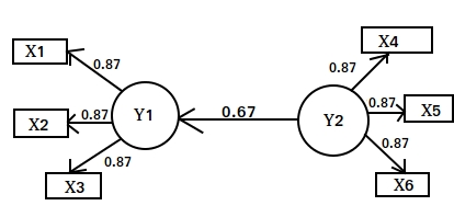
             Path Estimate
lam_1_1  y2 -> x4     0.87
lam_1_2  y2 -> x5     0.87
lam_1_3  y2 -> x6     0.87
lam_2_1  y1 -> x1     0.87
lam_2_2  y1 -> x2     0.87
lam_2_3  y1 -> x3     0.87
beta_1_2 y2 -> y1     0.67
So our results as visual model:

So I read in several papers that pls sem underestimates the inner model parameters and overestimates the outer model parameters. Those papers always cite
Schneeweiss, Hans. Consistency at large in models with latent variables. Amsterdam: Elsevier, 1993.
Unfortunately I could not find this paper anywhere until now and I don't know if I ever will get access to it.
In the previous example however I observed the same with the inner parameter going from 0.8 to 0.67 and the outer parameters from 0.8 to 0.87.
So is this really the cause of my observation? And if so, isn't that a really big difference for such a small model?
Or is there something conceptually wrong with my approach?
