7
$\begingroup$

After having a bit too much tea I decided to write a silly way of estimating the parameters of a single-feature linear regression. For starters, I avoided using techniques like gradient descent, least-squares, or a normal equation. I also didn't want to make the regression any more sophisticated by using feature scaling or regularization. Indeed, vectorization was intentionally avoided as well.

Despite my efforts to thwart validity, I think what I conjured up offers a suboptimal and inefficient, but not entirely ineffective, way to parametrize a linear model. I was able to fit it to some randomly generated data almost as well as least-squares, although I did find that it was outlier sensitive (which is expected from using averages).

Essentially, I used the two-point slope calculation for each data point with each subsequent datapoint, and took the arithmetic mean to estimate the slope. The error in the population slope was estimated with the standard deviation of the two-point slopes. Using each calculated slope with each data point, I calculate the intercept. The arithmetic mean of the calculated intercepts is used to estimate the population intercept, and the error was again estimated with the standard deviation.

As I see it, this is basically descriptive statistics done on multiple two-point estimates of parameters, but I want to know what others think.

What does this method of parametrization do invalidly, and validly? I would like to know what this method has been called if it has a name. What assumptions does this method make?

I've supplied the implementation for others to better understand the method, and to try it out if they want.

import numpy as np
import matplotlib.pyplot as plt

def regression(x, y, plot=False):

    slopes = []
    for i in range(len(y)):
        for j in range(len(y)):
            if (j>i):
                slopes.append((y[j] - y[i]) / (x[j] - x[i]))

    slopes_mean = np.mean(slopes)
    slopes_std = np.std(slopes)
            
    intercepts = []
    for slope in slopes:
        for i in range(len(y)):
            intercepts.append(y[i] - slope * x[i])
        
    intercepts_mean = np.mean(intercepts)
    intercepts_std = np.std(intercepts)

    residuals = []
    for slope in slopes:
        for intercept in intercepts:
            for i in range(len(y)):
                residuals.append((intercept + slope * x[i] - y[i])**2)

    residual_error = sum(residuals)

    if plot == True:
        plt.scatter(x,y,color='k')
        plt.plot([i for i in np.arange(min(x),max(x) + 1)],[i*np.mean(slopes) + np.mean(intercepts) for i in np.arange(min(x),max(x) + 1)], color='r')
        plt.xlabel('x')
        plt.ylabel('y')
        plt.show()
    
    return slopes_mean, slopes_std, intercepts_mean, intercepts_std, residual_error

Observations

The values of y are predicted exactly by the model when the sample points make a straight line.

The estimated parameters by this method were not much different than those parametrized by scipy.stats.linregress().

The estimated parameters were not far off from the true parameters of a simulated dataset with Gaussian noise added.

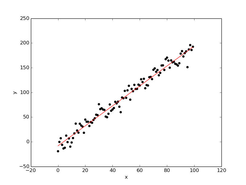
Parametrized Model Fit to Gaussian Line

$\endgroup$
8
  • $\begingroup$ What was in the tea ? In my opinion what your approach doesn't do is to estimate the parameters that have the greatest likelihood / chance of being the true values. $\endgroup$
    – IrishStat
    Commented Aug 10, 2015 at 0:56
  • $\begingroup$ It was Earl Grey, if that explains it. So, you think the method has a bias? Would you explain? $\endgroup$
    – Galen
    Commented Aug 10, 2015 at 1:11
  • $\begingroup$ @Galen Why not use all possible pairs instead of just the adjacent points (at least I think that's how you did it)? Seems like the all possible pairs approach might be a bit more "robust." Of course this wouldn't work very well with big data sets. $\endgroup$
    – dsaxton
    Commented Aug 10, 2015 at 1:16
  • $\begingroup$ @dsaxton For each point, it calculates the slope with all subsequent points, which are not necessarily adjacent. Doing this prevents calculating the slope for the same two points as the programs loops over all the points. $\endgroup$
    – Galen
    Commented Aug 10, 2015 at 1:20
  • 2
    $\begingroup$ You might find Theil regression interesting. For its slope estimate, it uses the median of pairwise slopes across all pairs (with distinct x). It also corresponds to making Kendall's tau between residuals and the x-variable equal to zero. $\endgroup$
    – Glen_b
    Commented Aug 10, 2015 at 5:37

1 Answer 1

10
$\begingroup$

Assuming:

  • $x_i$ and $x_j$ must always be distinct (for simplicity; otherwise the calculations require us to keep conditioning on the distinct pairs and I'd rather leave that out for now)

  • $y=\beta_0+\beta_1 x+\varepsilon$, with $E(\varepsilon)=0$

  • $x$'s fixed not random

then the pairwise slopes have expectation $\beta_1$, since:

$E(y_j-y_i) = E[\beta_0+\beta_1 x_i+\varepsilon_j - (\beta_0+\beta_1 x_i+\varepsilon_i)]$

$\qquad = \beta_1(x_j-x_i)$

And consequently so will an average of these individual pairwise estimates. So it's unbiased.

Actually this wasn't surprising, since OLS is actually a weighted average of those pairwise slopes.

e.g. see Sanford Weisberg's Applied Linear Regression, 4E sec 2.11.2

Also see Gelman's blog here.

We could look at variance (there's several ways to approach this); I'll outline a simple-minded approach but I haven't time to carry it all through right now.

For this we further assume the $\varepsilon$'s are independent with constant variance $\sigma^2$.

$\text{Var}(y_j-y_i) =\varepsilon_j+\varepsilon_i=2\sigma^2$, so

$\text{Var}b_{ij}=\text{Var}\frac{y_j-y_i}{x_j-x_i} =2\frac{\sigma^2}{(x_j-x_i)^2}$

OLS weights each slope $b_{ij}$ by $\frac{(x_j-x_i)^2}{2nS_{xx}}$ -- which is to say, observations that are further apart get more weight (as they should, since the variance of their slope estimate is smaller).

Since your estimator doesn't weight its average, the variance will be larger, but given that the point was to arrive at a conceptually "simple" estimator, we shouldn't quibble too much about efficiency.

The next step would be to try to compute the variance of the overall estimator of slope. Here we could just rely on basic properties of variance.

$\text{Var}(\sum_{ij} b_{ij}) = \sum_{ij} \text{Var}(b_{ij}) + \sum_{(i,j)\neq (k,l)}\text{Cov}(b_{ij},b_{kl})$

However, only those terms where $i$ or $j$ occurs twice will have nonzero covariance. I believe there are three cases to worry about: $k=i, k=j, l=j$ (other coincident pairings being covered by doubling in the usual fashion)


As a more concrete aside, consider a case with 4 points $(A,B,C,D)$ -- there are 15 (i.e. $ \binom{\binom {4} {2}}{2}$) pairs of slopes (themselves indexed as pairs) of which these pairs count for covariance:

AB AC
AB AD
AC AD
BC BD

AB BC
AB BD
AC CD
BC CD

AC BC
AD BD
AD CD
BD CD

and these don't count for covariance:

AB CD 
AC BD 
AD BC

(That's what I'm attempting to outline the general case of...)

$\qquad = 2\sigma^2\sum_{ij} \frac{1}{(x_j-x_i)^2} + 2\sum_{i<j<l}\text{Cov}(b_{ij},b_{il})+2\sum_{i<j<l}\text{Cov}(b_{ij},b_{jl})$
$\qquad\qquad+2\sum_{i<k<j}\text{Cov}(b_{ij},b_{kj})$

(I hope I have that right!)

from there it's just a matter of plugging through the usual basic linearity properties for covariances (making use of the fact that the x's are constant, and the epsilons are independent except when they're the same, when things reduce to a variance). Nothing is especially onerous.

I may come back and try to finish that when I get a chance, but it may well be easier to see if one can write this in the form $\hat{\beta}=Ay$ and derive the variance that way (I was attempting to avoid matrix calculations to remain in the spirit of 'derp regression' but the matrix approach might save effort). actually since we only have one beta coefficient, $A$ would be a vector of partials, $A=a'=\frac{\partial \hat{\beta_1}}{\partial y_k}$, which would be convenient to write in the form $q1'W$ where $q$ is a scaling factor, $1$ is a vector of ones and $W$ is a matrix of "weight" coefficients of the form $W_{ij}=\frac{1}{x_j-x_i}$ (for $i\neq j$, and $0$ otherwise).

The efficiency of this relative to OLS depends on the pattern of $x$'s. If the $x$'s have very small "kurtosis" (all the x's are at the very ends of the range of $x$ so all or almost all non-zero x-differences are large) then it will be highly efficient. If there's an abundance of small x-differences, then it will be much less efficient.

It occurs to me that papers on Theil regression already explore some of those notions (with similar conclusions relevant to efficiency).


There's also a connection to Theil regression here. For its slope estimate, it uses the median of pairwise slopes across all pairs (with distinct x). It also corresponds to making Kendall's tau between residuals and the x-variable equal to zero.

Here's some very simple-minded code for producing a median of pairwise slopes in R:

theilb = median(outer(y,y,"-")/outer(x,x,"-"),na.rm="TRUE")

of course substantially more efficient calculations can be arranged (this takes twice as long as even a sensible $O(n^2)$ calculation, and $O(n \log n)$ calculations are possible, though I can't say I've ever attempted to write them -- the papers on efficient calculations of this seem pretty heavy going).

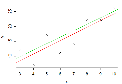
Here's a comparison of the two on a small data set (your slope in red, Theil in green). The main difference in this particular example is in the estimate of intercept (I just used mean and median residual respectively).

enter image description here

$\endgroup$

Your Answer

By clicking “Post Your Answer”, you agree to our terms of service and acknowledge you have read our privacy policy.

Not the answer you're looking for? Browse other questions tagged or ask your own question.