Interpreting group differences in an ANCOVA
The value of an ANCOVA model is that it allows you to test for group differences after controlling for a covariate. This is only worthwhile if the covariate matters. So the fact that you see a strong relationship between your DV and your covariate isn't necessarily a problem. The issue here is that the interpretation of group differences in an ANCOVA is really different from the interpretation of group differences in an ANOVA. By including a covariate, you're no longer testing for overall differences in the DV by group; you're only testing for differences in the group means after adjusting for the covariate (the estimated marginal means).
A quick example to illustrate: Let's say you're testing the effectiveness of a weight loss program. You randomly assign pariticipants to either your weight loss program or a control group. At the end you measure their weight. Now, if you tried to test the effectiveness of your program by just comparing the end weights of people in your program vs. the control, that would be silly --- their weight at the end of the program will be strongly related to their weight going into the program! Just examining the end weights could be misleading. For example, if it just so happened that folks randomly assigned to your program were lighter on average to begin with, then showing that they're lighter at the end doesn't necessarily mean anything. What you really want to do is to look at their weights at the end of the study controlling for their weights going in, i.e. the change in weight. This is a case where an ANCOVA is a great model, because you know there's an important covariate (weight before starting the program) and you want to look at the effect of group assignment (treatment vs. control) after controlling for that covariate.
You asked:
Does it mean that the manipulated variables do only have a minor effect on the dependent variable and explain much less than the covariate? If so, is the experiment actually useless as the manipulated variables barely explain variance of the dependent variable?
What it means is that you're asking a different question than you ask in an ANOVA. With an ANCOVA, you're looking for differences in the estimated marginal means (aka conditional means, adjusted means, or least-squares means, depending on the software you're using and your field). You're generally not asking whether the covariate or the grouping variable(s) are more important. Instead, you're assuming that the covariate is important, and you're partialing it out so that you can look at the group differences after removing the covariate's effect from the data.
The second part of this question ("is the experiment actually useless") is really a question about effect sizes.
How to tell if your effects matter
Significance tests (i.e. your p values) depend strongly on sample size. It can be very hard to tell whether, for example, the group differences you're seeing are meaningful by looking at significance tests alone. I encourage you to look at effect size estimates (e.g. partial $\eta^2$) in addition to significance tests, so that you can get a better sense for how big these differences actually are.
Similarly, plotting your data can provide a great reality check, especially in cases where the effects are harder to interpret from the numbers alone (such as interpreting group differences in an ANCOVA vs. an ANOVA, as you point out).
Example code and output in R
(Note that some of the output has been truncated to keep the post more readable.)
# set the random seed
set.seed(8675309)

# generate some toy data
pre_weight <- rnorm(100, mean = 150, sd = 10)
group <- gl(2, k=50, labels = c("Treatment", "Control"))
post_weight <- pre_weight + ifelse(group == "Treatment", -10, 0) + rnorm(100, sd = 10)
Since we have an ANCOVA in mind, test the assumption of homogeneity of slopes:
> m1 <- lm(post_weight ~ pre_weight + group)
> m2 <- lm(post_weight ~ pre_weight * group)
> anova(m1, m2)
Analysis of Variance Table

Model 1: post_weight ~ pre_weight + group
Model 2: post_weight ~ pre_weight * group
  Res.Df    RSS Df Sum of Sq      F Pr(>F)
1     97 9617.2
2     96 9557.1  1    60.018 0.6029 0.4394
It looks like the assumption is met (i.e. there's no interaction between the covariate and the grouping variable), which is unsurprising since I generated the data as an ANCOVA example. ;)
Check out the results of an ANOVA analysis and an ANCOVA analysis, like you did your question:
> summary(lm(post_weight ~ group)) # ANOVA

Coefficients:
             Estimate Std. Error t value Pr(>|t|)
(Intercept)   141.358      1.982  71.316   <2e-16 ***
groupControl    7.314      2.803   2.609   0.0105 *
---
Signif. codes:  0 ‘***’ 0.001 ‘**’ 0.01 ‘*’ 0.05 ‘.’ 0.1 ‘ ’ 1

Residual standard error: 14.02 on 98 degrees of freedom
Multiple R-squared:  0.06495,   Adjusted R-squared:  0.05541
F-statistic: 6.808 on 1 and 98 DF,  p-value: 0.0105

> summary(lm(post_weight ~ pre_weight + group)) # ANCOVA

Coefficients:
             Estimate Std. Error t value Pr(>|t|)
(Intercept)  -19.2300    16.3514  -1.176    0.242
pre_weight     1.0633     0.1079   9.858 2.72e-16 ***
groupControl   8.3855     1.9944   4.205 5.83e-05 ***
---
Signif. codes:  0 ‘***’ 0.001 ‘**’ 0.01 ‘*’ 0.05 ‘.’ 0.1 ‘ ’ 1

Residual standard error: 9.957 on 97 degrees of freedom
Multiple R-squared:  0.5329,    Adjusted R-squared:  0.5233
F-statistic: 55.33 on 2 and 97 DF,  p-value: < 2.2e-16
These data are similar to yours in that including the covariate makes a big difference ($R^2$ jumps from .06 in the ANOVA to .53 in the ANCOVA). Let's break that down.
Get effect size estimates to measure the importance of the grouping variable in the ANCOVA model. Partial eta squared is pretty easy to calculate by hand if you have the sums of squares for each effect, so that's how I usually do it. There's probably a package that provides a nice function for this, though, if you prefer.
# getting the sums squared for each effect using the Anova function from the car package
sstable <- car::Anova(lm(post_weight ~ pre_weight + group), type = 3)
# partial eta squared:
sstable$pes <- c(sstable$'Sum Sq'[-nrow(sstable)], NA)/(sstable$'Sum Sq' + sstable$'Sum Sq'[nrow(sstable)]) # SS for each effect divided by the last SS (SS_residual)
This produces a nice-looking table that inlcudes partial eta squared for each effect:
> sstable
Anova Table (Type III tests)

Response: post_weight
            Sum Sq Df F value   Pr(>F)     pes
(Intercept)  137.1  1  1.3831 0.242453 0.01406
pre_weight  9634.4  1 97.1743 0.000000 0.50045
group       1752.7  1 17.6778 0.000058 0.15415
Residuals   9617.2 97
This shows that, yes, the covariate has a big effect, but the grouping variable also has a pretty sizable effect in the ANCOVA. What counts as a "big" effect varies a lot by context (and research field), but .15 is definitely nothing to sneeze at in the social sciences (where I got my training).
Remember that this test of group differences is asking a fundamentally different question from the test in the ANOVA; you're measuring weight loss here, not just overall weight at the end of the study.
Note there are lots of other estimates of effect size you could consider here, and pros and cons of each. Here is a nice CV post to get your started on some of those considerations.
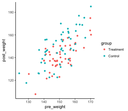
Plot it:
library(ggplot2)

my_data <- data.frame(pre_weight, group, post_weight)

p <- ggplot(my_data, aes(y=post_weight, x=pre_weight, color = group, fill = group)) +
  geom_point() +
  theme_classic()
This plot (p) is just a scatterplot of all of the participants in my (made-up) weight loss study. They are colored by group assignment, but as you can see, their weight at the end of the study is largely a function of their weight coming in.

We can add regression lines for each group with stat_smooth:
p + stat_smooth(method = "lm")

This helps to make clear that while pre_weight has a large predictive effect for post_weight (the slopes of both lines are clearly non-zero), there is also an effect of group assignment: People assigned to the treatment group have a lower post_weight after controlling for pre_weight than people in the control group do (the regression line for Treatment is lower than for Control).


