Generating Double-Triangular-distributed random variates

Question

Wikipedia shows how to generate Triangular-distributed random variates using a variate $U$ drawn from the uniform distribution.

A "Double Triangular" distribution is a special case of a mixture of two triangular distributions. Specifically, it is determined by three numbers $a \lt c \lt b$ and a proportion $p$ with $0 \lt p \lt 1$. It is supported on the interval $[a, b]$.

On the interval $[a,c]$ its density function is given by

$$f(x) = \lambda(x-a)$$

where $\lambda(c-a)^2 = 2p$.

On the interval $[c, b]$ its density function is given by

$$f(x) = \mu(b-x)$$

where $\mu(b-c)^2 = 2(1-p)$.

What would be a good approach to generating Double-Triangular-distributed random variates?

Answer 1

Following whuber's comments, here is a way to simulate from the mixture using a single uniform:

Since the pdf of this mixture is $$f(x)=p\dfrac{2(x-a)}{(c-a)^2}\mathbb{I}_{(a,c)}(x)+(1-p)\dfrac{2(b-x)}{(b-c)^2}\mathbb{I}_{(c,b)}(x)$$ the cdf is$$F(x)=p\dfrac{(x-a)^2}{(c-a)^2}\mathbb{I}_{(a,c)}(x)+\left\{p+(1-p)\left[1-\dfrac{(b-x)^2}{(b-c)^2}\right]\right\}\mathbb{I}_{(c,b)}(x)+\mathbb{I}_{(b,\infty)}(x)$$ Drawing a single uniform $U\sim\mathcal{U}(0,1)$ and inverting the equation$$u=p\dfrac{(x-a)^2}{(c-a)^2}\mathbb{I}_{(a,c)}(x)+\left\{p+(1-p)\left[1-\dfrac{(b-x)^2}{(b-c)^2}\right]\right\}\mathbb{I}_{(c,b)}(x)$$produces a generation of $X\sim f(x)$. This inversion can be decomposed into two steps:

1. Determine if $u\le p$ or $u>p$ [this is the decomposition of the uniform suggested by whuber]
2. If $u\le p$, solve $(x-a)^2=(u/p)(c-a)^2$, namely take $$x=a+\sqrt{u/p}(c-a)$$
3. Else, if $u>p$, set $v=(u-p)/(1-p)$ and solve $(b-x)^2=(1-v)(b-c)^2$, namely take $$x=b-\sqrt{1-v}(b-c)$$or equivalently$$x=b-\sqrt{v}(b-c)$$

Interestingly, the last equation is not equivalent to $$x=c+\sqrt{1-v}(b-c)$$because of the squared root.

Answer 2

Rejection sampling is quite simple here (see the accepted answer or the end of this post for more efficient alternatives, though):

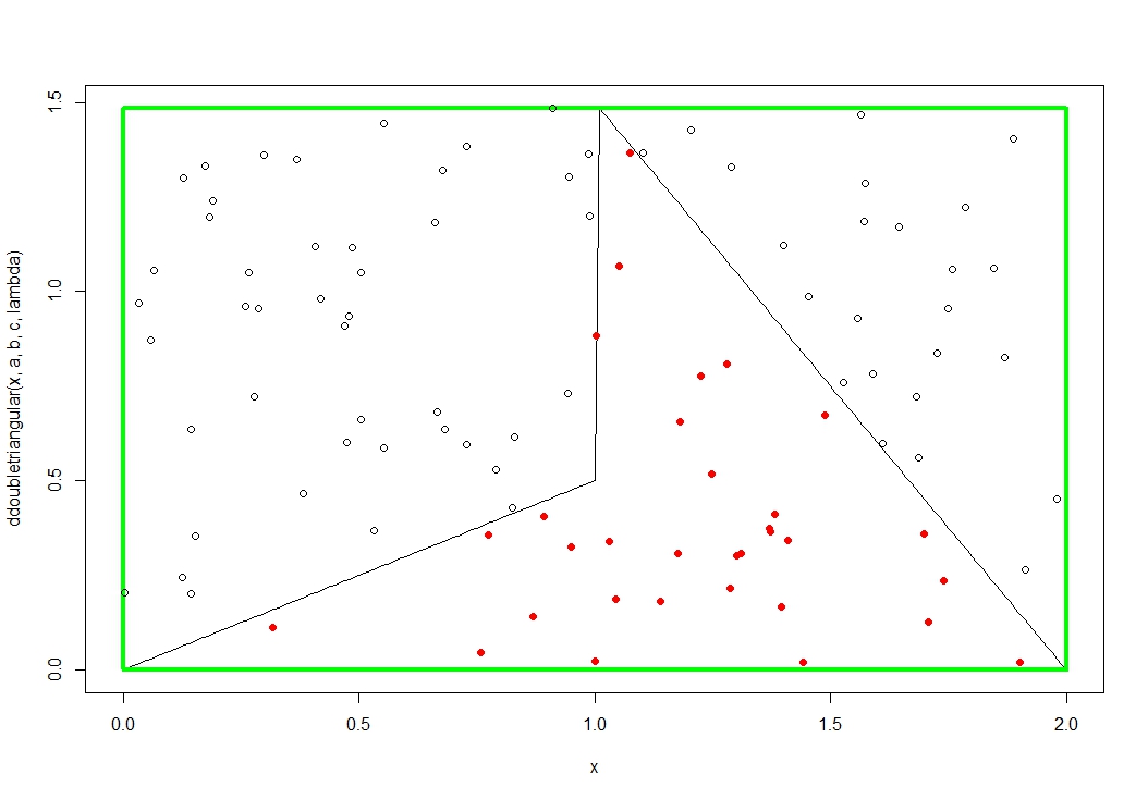
1. Build a rectangle around the density (which is easy here due to bounded support) - the green box in the figure.
2. Draw uniform variates in the box (so just two uniform vectors with the right suppport in both directions) - all the dots in the figure, both blank and red.
3. Keep those points which are below the density of the double triangular (the red dots in the figure).
4. Take the "$x$-axis" coordinates of these points as realizations of the double triangular.

In a picture:

Created with

a <- 0
b <- 2
c <- 1
lambda <- .5
x <- seq(a,b,by=.01)
ddoubletriangular <- function(x,a,b,c,lambda){
  p <- lambda/2*(c-a)^2
  mu <- 2*(1-p)/(b-c)^2
  return(lambda*(x-a)*(x<=c)+mu*(b-x)*(x>c))
}
plot(x,ddoubletriangular(x,a,b,c,lambda),type="l")
upperbound <- max(ddoubletriangular(x,a,b,c,lambda))
lines(c(b,b,a,a,b),c(0,upperbound,upperbound,0,0),col="green",lwd=4)

px <- runif(100,min=a,max=b)
py <- runif(100,min=0,max=upperbound)
points(px,py)

ikeep <- (py < ddoubletriangular(px,a,b,c,lambda))
px <- px[ikeep]
py <- py[ikeep]
points(px,py,col="red",pch=19)  

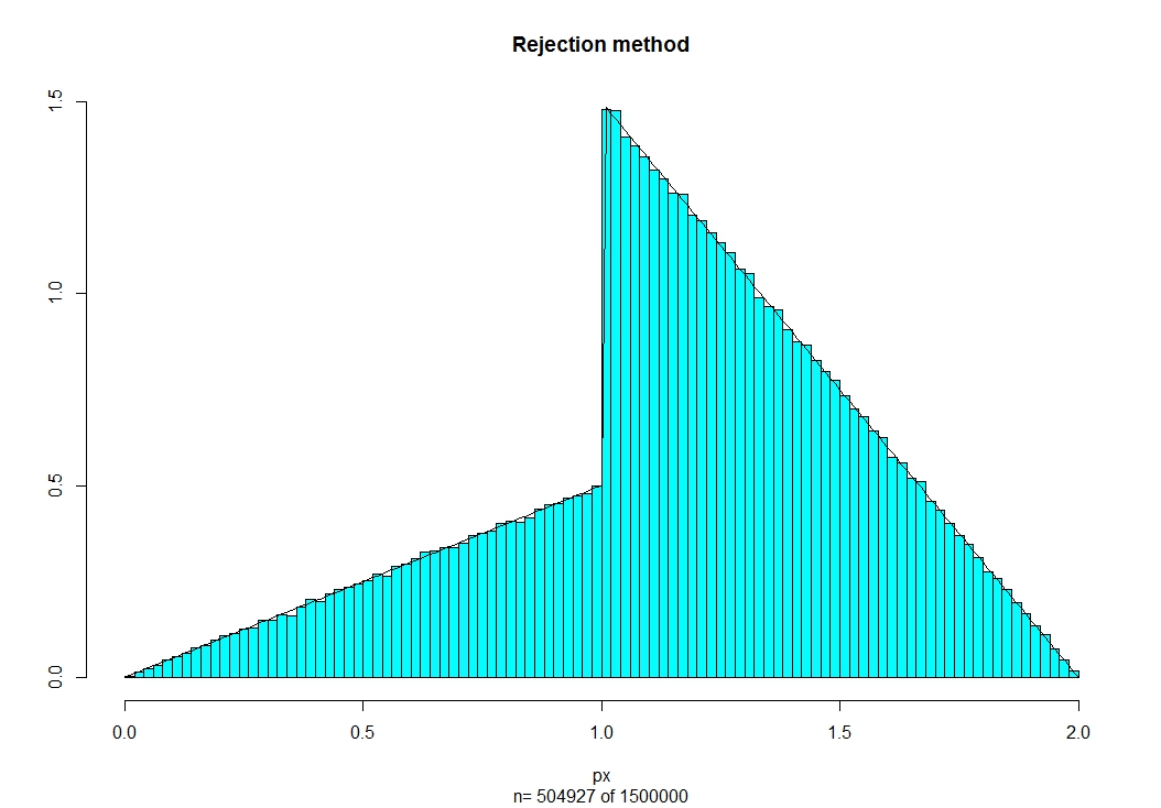
Let's try more than just $N=100$ draws to study the quality of the algorithm:

N <- 1500000
px <- runif(N,min=a,max=b)
py <- runif(N,min=0,max=upperbound)
ikeep <- (py < ddoubletriangular(px,a,b,c,lambda))
px <- px[ikeep]
truehist(px,main="Rejection method",sub=paste("n=",length(px),"of",N))
lines(x,ddoubletriangular(x,a,b,c,lambda),type="l")

This results in

UPDATE:

As forcefully documented in the comments, the above algorithm is, being "off-the shelf", unnecessarily inefficient. Here is an illustration of what @whuber proposes (or so I hope):

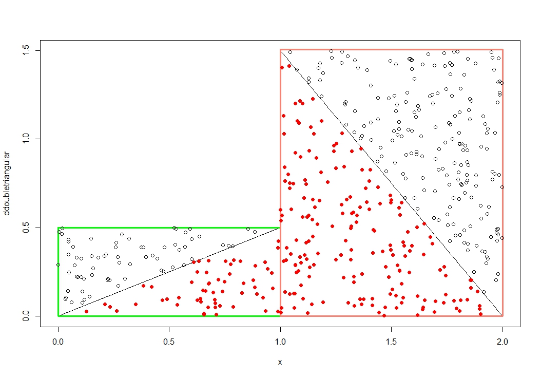
First improvement:

Build two rectangular boxes and perform rejection sampling in each region separately (with probability $p$ for the first segment, and $1-p$ for the second), see the next figure. This by construction improves the acceptance probability to 1/2.

Second improvement:

Recognize that the regions in the boxes each are what @whuber calls "rectangular symmetric": the triangle above a segment of the linear density is a rotated version of the acceptance triangle below the density. Hence, we may use the "rejected" samples of the basic algorithm and use these as legitimate realizations for the other end of the segment.

For example, a rejected draw with $x$-coordinate $c+\epsilon$ may be used as an accepted draw for $b-\epsilon$, because the "height" of the rejection region at $c+\epsilon$ is by construction identical to the "height" of the acceptance region at $b-\epsilon$. This has the nice feature of increasing the acceptance rate to 100%.

Here is a way to code that:

a <- 0
b <- 2
c <- 1
lambda <- .5
x <- seq(a,b,by=.002)
p <- lambda/2*(c-a)^2
mu <- 2*(1-p)/(b-c)^2
ddoubletriangular <- lambda*(x-a)*(x<=c)+mu*(b-x)*(x>c)

upperbound1 <- lambda*c
upperbound2 <- mu*x[min(which(x>c))+1]

N <- 1500000
px1 <- runif(N*p,min=a,max=c)
py1 <- runif(N*p,min=0,max=upperbound1)

px2 <- runif(N*(1-p),min=c,max=b)
py2 <- runif(N*(1-p),min=0,max=upperbound2)

ikeep1 <- (py1 < lambda*(px1-a))
px1a <- px1[ikeep1]
px1b <- a+c-px1[!ikeep1]

ikeep2 <- (py2 < mu*(b-px2))
px2a <- px2[ikeep2]
px2b <- c+b-px2[!ikeep2]

px <- c(px1a,px1b,px2a,px2b)

truehist(px,main="Modified rejection method",sub=paste("n=",length(px),"of",N))
lines(x,lambda*(x-a)*(x<=c)+mu*(b-x)*(x>c),type="l")