GP regression with high-dimensional time-series data

Question

I have what I think is a neat little problem which involves regression. My observations are somewhat sparse, and they are very high-dimensional (though this can be probably be reduced by a factor of say 10-15 quite easily).

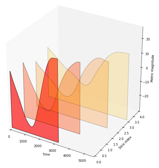
For an illustration of my data, please see here:

Just to be clear; the data itself is the top edge of each face (the face is really just there for illustration purposes). You will also note that the inputs are of different dimensionality (this is not a problem either; it can be dealt with using interpolation).

BUT what I am wondering is; is it sensible to try to use GPs to basically regress the regions between these faces? As you can see there is a clear correlation between index, time and the metric itself. But because I am quite uncertain about the regions in between the faces, I thought that using GPs could be a good idea.

What I have then is:

$\mathbf{x} = f(\mathbf{Y}) + \epsilon$

where we can consider the structure of the inputs to be:

$\mathbf{Y} = \begin{bmatrix}[y_1,\ldots,y_k]\\ \vdots \\ [y_1,\ldots,y_k]\end{bmatrix}$

where the $\mathbf{Y}$ has $N$ rows (observations) and $K$ columns (dimensions).

And the target value would just be an index (so a many-to-one mapping).

Now as you can see from the figure, there are a lot of dimensions (the time axis on the figure above) - because I would like to capture the overall shape of the curve as it goes from index to index.

What I am really wondering, I suppose, is whether this is a suitable problem for GPs? Further, it is also fully possibly, to simply use a second or third-order polynomial to interpolate between the curves.

Answer 1

The following problem is identical to yours, might be helpful.

import numpy as np
import pylab as plt
import seaborn as snb
import GPy
from pyDOE import*
from scipy.stats.distributions import norm

tend = 3000
time = np.arange(tend)[:,None]
ns = 100
xdata = np.load('xdata%d.npy'%ns)
ydata = np.load('ydata%d.npy'%ns)

xtest = np.load('xdata_T8.npy')
ytest = np.load('ydata_T8.npy')

nt = 30
tpoints = np.linspace(0,tend-1,nt,dtype='int64')
timeStack = np.tile(tpoints,ns)
xdataStack = np.repeat(xdata,nt, axis=0)

xtrain = np.c_[xdataStack, timeStack]
ytrain = ydata[:, tpoints]
ytrain = ytrain.flatten()[:,None]

se = GPy.kern.RBF(6,1,10)
ln1 = GPy.kern.Linear(6)
ln2 = GPy.kern.Linear(6)
rq = GPy.kern.RatQuad(6)
kernel = se*(ln1+ln2*rq)
m = GPy.models.GPRegression(xtrain,ytrain,kernel)
m.optimize()

n = 1000
nt = 300

tpoints = np.linspace(0,tend-1,nt,dtype='int64')[:,None]
mu = np.zeros((n,nt))
var = np.zeros((n,nt))

fig = plt.figure(figsize=(6.5, 6))
for i in range(n):
    ixtest = xtest[i,:][:,None].T
    ixtest = np.repeat(ixtest,nt,axis=0)
    ixtest = np.column_stack((ixtest, tpoints))
    muu,varr = m.predict(ixtest)
    mu[i,:][:,None] = muu
    var[i,:][:,None] = varr
    if (i==0):
        plt.plot(tpoints,mu[i,:],'b-',markersize=2, alpha =1, label = 'Gaussian Model',linewidth=2)
        plt.plot(tpoints,mu[i,:]+2*np.sqrt(var[i,:]),'r--',label = 'Uncertainty Bounds', alpha =0.5,linewidth=2)
        plt.plot(tpoints,mu[i,:]-2*np.sqrt(var[i,:]),'r--',markersize=2, alpha =0.5,linewidth=2)
        plt.plot(tpoints,ytest[i,tpoints],'k-',markersize=2, alpha = 1, label = 'FEM Model',linewidth=2)
    else:
        plt.plot(tpoints,mu[i,:],'b-',markersize=2, alpha =1,linewidth=2)
        plt.plot(tpoints,mu[i,:]+2*np.sqrt(var[i,:]),'r--',markersize=2, alpha =0.5,linewidth=2)
        plt.plot(tpoints,mu[i,:]-2*np.sqrt(var[i,:]),'r--',markersize=2, alpha =0.5,linewidth=2)
        plt.plot(tpoints,ytest[i,tpoints],'k-',markersize=2, alpha = 1,linewidth=2)
plt.legend(loc =4)
plt.xlabel('Time, t[s]')
plt.ylabel('[$^\circ $C]')
plt.title('Wall Temperatures')
plt.show()