From your description, I have no idea what you did. It doesn't sound right, but it's hard to say. Here is how I'd analyze your data:
d = read.table(text="  Dose Cells Dicentrics Laboratory Culture
                        0.1 328 2 Edinburgh Immediate
                        ...
                        3.0 291 46 Pittsburgh Stored", header=T)
The first thing to notice is that these are binomial data. That is, they are counts of 'successes' out of a known total number of 'trials'. You need to use a logistic regression model here. I start with a full model with all interactions (in part because I have no idea what this is), and I include a squared effect of Dose (because you seem to want that).
m = glm(cbind(Dicentrics, Cells-Dicentrics)~poly(Dose,2)*Culture*Laboratory,
        d, family=binomial)
summary(m)
# output omitted
We can use analysis of deviance tests (i.e., a likelihood ratio test of a nested model) to test the three-way interaction and the need for the squared term:
anova(update(m, .~poly(Dose,1)*Culture*Laboratory, d), m, test="LRT")
# Analysis of Deviance Table
#
# Model 1: cbind(Dicentrics, Cells - Dicentrics) ~ poly(Dose, 1) + Culture +
#     Laboratory + poly(Dose, 1):Culture + poly(Dose, 1):Laboratory +
#     Culture:Laboratory + poly(Dose, 1):Culture:Laboratory
# Model 2: cbind(Dicentrics, Cells - Dicentrics) ~ poly(Dose, 2) * Culture *
#     Laboratory
#   Resid. Df Resid. Dev Df Deviance  Pr(>Chi)
# 1        20     65.812
# 2        16      6.457  4   59.355 3.963e-12 ***
# ---
# Signif. codes:  0 ‘***’ 0.001 ‘**’ 0.01 ‘*’ 0.05 ‘.’ 0.1 ‘ ’ 1
anova(update(m, .~.-poly(Dose,2):Culture:Laboratory, d), m, test="LRT")
# Analysis of Deviance Table
#
# Model 1: cbind(Dicentrics, Cells - Dicentrics) ~ poly(Dose, 2) + Culture +
#     Laboratory + poly(Dose, 2):Culture + poly(Dose, 2):Laboratory +
#     Culture:Laboratory
# Model 2: cbind(Dicentrics, Cells - Dicentrics) ~ poly(Dose, 2) * Culture *
#     Laboratory
#   Resid. Df Resid. Dev Df Deviance Pr(>Chi)
# 1        18     6.6571
# 2        16     6.4569  2  0.20016   0.9048
You seem to be right about the need for a polynomial fit, but there really doesn't seem to be any need for the three-way interaction.
At this point, modeling philosophies diverge: many will drop the interaction, but some advise against it. I am generally uncomfortable with dropping variables just because they are not significant, but this is sufficiently non-significant that I don't see much problem. In particular, dropping the interaction can make testing and interpreting the model simpler.
m2 = glm(cbind(Dicentrics, Cells-Dicentrics)~(poly(Dose,2)+Culture+Laboratory)^2,
         d, family=binomial)
summary(m2)
# output omitted
This fits a model with three two-way interactions, but not the three-way. We can conduct subsequent tests of these two-way interactions.
anova(update(m2, .~.-poly(Dose,2):Culture, d), m2, test="LRT")
# Analysis of Deviance Table
#
# Model 1: cbind(Dicentrics, Cells - Dicentrics) ~ poly(Dose, 2) + Culture +
#     Laboratory + poly(Dose, 2):Laboratory + Culture:Laboratory
# Model 2: cbind(Dicentrics, Cells - Dicentrics) ~ (poly(Dose, 2) + Culture +
#     Laboratory)^2
#   Resid. Df Resid. Dev Df Deviance Pr(>Chi)
# 1        20    12.9341
# 2        18     6.6571  2    6.277  0.04335 *
# ---
# Signif. codes:  0 ‘***’ 0.001 ‘**’ 0.01 ‘*’ 0.05 ‘.’ 0.1 ‘ ’ 1
anova(update(m2, .~.-poly(Dose,2):Laboratory, d), m2, test="LRT")
# Analysis of Deviance Table
#
# Model 1: cbind(Dicentrics, Cells - Dicentrics) ~ poly(Dose, 2) + Culture +
#     Laboratory + poly(Dose, 2):Culture + Culture:Laboratory
# Model 2: cbind(Dicentrics, Cells - Dicentrics) ~ (poly(Dose, 2) + Culture +
#     Laboratory)^2
#   Resid. Df Resid. Dev Df Deviance Pr(>Chi)
# 1        20    12.0733
# 2        18     6.6571  2   5.4163  0.06666 .
# ---
# Signif. codes:  0 ‘***’ 0.001 ‘**’ 0.01 ‘*’ 0.05 ‘.’ 0.1 ‘ ’ 1
anova(update(m2, .~.-Culture:Laboratory, d), m2, test="LRT")
# Analysis of Deviance Table
#
# Model 1: cbind(Dicentrics, Cells - Dicentrics) ~ poly(Dose, 2) + Culture +
#     Laboratory + poly(Dose, 2):Culture + poly(Dose, 2):Laboratory
# Model 2: cbind(Dicentrics, Cells - Dicentrics) ~ (poly(Dose, 2) + Culture +
#     Laboratory)^2
#   Resid. Df Resid. Dev Df Deviance Pr(>Chi)
# 1        19     7.5582
# 2        18     6.6571  1   0.9011   0.3425
Here we see that there seems to be a Dose by Culture interaction (which I suspect makes scientific sense), no evidence of a Culture by Laboratory interaction (which also seems plausible), and a Dose by Laboratory interaction that doesn't quite meet the traditional criterion for 'statistical significance' (I'm not sure whether its existence makes sense). Although a p-value of $0.34$ might be kind of low, the observed value of the test statistic is $0.9$, which is less than the expected value of a $\chi^2$ random variable on $1$ df. I am slightly uncomfortable with dropping this, but willing to do so in the name of enhanced simplicity and interpretability. I would not drop the Dose by Laboratory interaction, however. (So the model remains somewhat harder to interpret.) The existence of the interaction that includes Laboratory implies that it is potentially relevant.
Here I fit the final model:
m3 = glm(cbind(Dicentrics, Cells-Dicentrics)~poly(Dose,2)*Laboratory+
                                             poly(Dose,2)*Culture,
         d, family=binomial)
summary(m3)
# Call:
# glm(formula = cbind(Dicentrics, Cells - Dicentrics) ~ poly(Dose,
#     2) * Laboratory + poly(Dose, 2) * Culture, family = binomial,
#     data = d)
#
# Deviance Residuals:
#     Min       1Q   Median       3Q      Max
# -1.1235  -0.3427   0.1043   0.3425   0.9214
#
# Coefficients:
#                                     Estimate Std. Error z value Pr(>|z|)
# (Intercept)                          -4.2729     0.1682 -25.405   <2e-16 ***
# poly(Dose, 2)1                        6.7074     0.8008   8.376   <2e-16 ***
# poly(Dose, 2)2                       -0.7665     0.6117  -1.253   0.2101
# LaboratoryPittsburgh                  0.2929     0.1786   1.641   0.1009
# CultureStored                         0.2206     0.1849   1.193   0.2328
# poly(Dose, 2)1:LaboratoryPittsburgh  -1.0325     0.8358  -1.235   0.2167
# poly(Dose, 2)2:LaboratoryPittsburgh  -0.4245     0.5749  -0.738   0.4603
# poly(Dose, 2)1:CultureStored          2.1885     0.8796   2.488   0.0128 *
# poly(Dose, 2)2:CultureStored         -1.3988     0.6500  -2.152   0.0314 *
# ---
# Signif. codes:  0 ‘***’ 0.001 ‘**’ 0.01 ‘*’ 0.05 ‘.’ 0.1 ‘ ’ 1
#
# (Dispersion parameter for binomial family taken to be 1)
#
#     Null deviance: 759.2740  on 27  degrees of freedom
# Residual deviance:   7.5582  on 19  degrees of freedom
# AIC: 132.86
#
# Number of Fisher Scoring iterations: 4
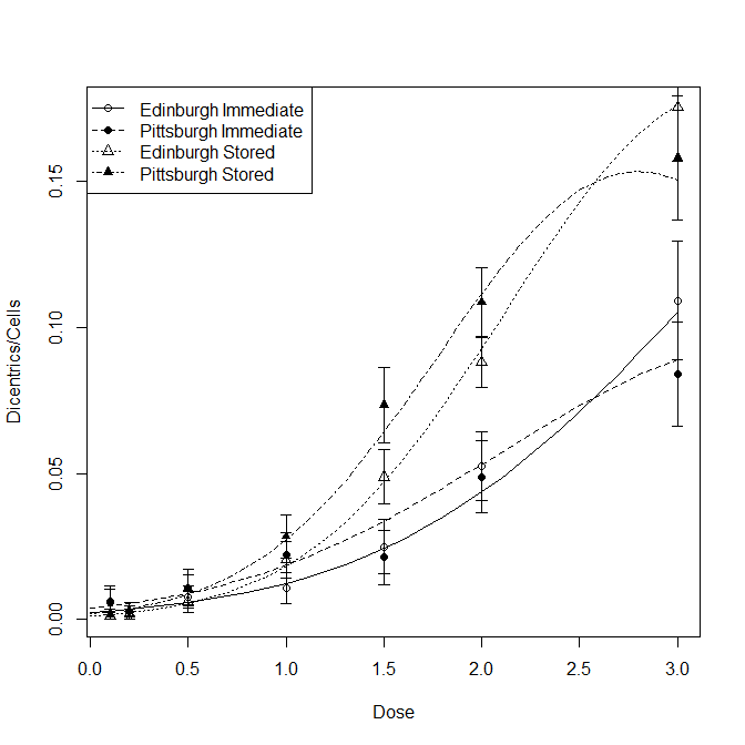
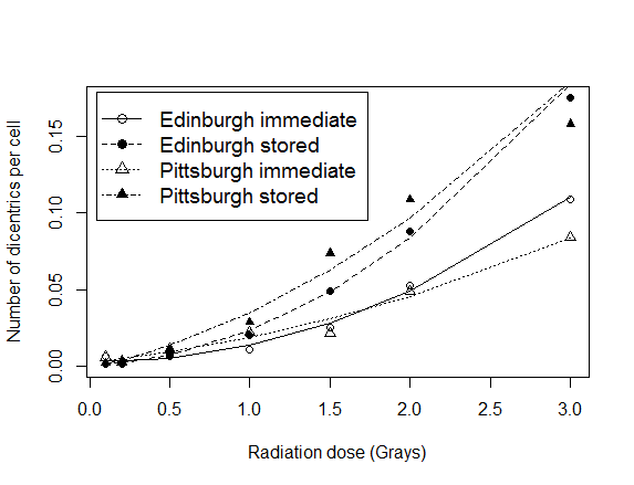
To evaluate and interpret this model, I make a plot of the data with the model's predicted values overlaid. To get a quick sense of the variability associated with each point (proportion dicentric), I compute the normal approximation of the binomial's standard error and plot that for each point as well.
xseq = seq(0,3, by=.1)
prop = with(d, Dicentrics/Cells)
pSE  = with(d, sqrt(prop*(1-prop)/Cells))

pchs = with(d, ifelse(Laboratory=="Edinburgh"&Culture=="Immediate",   1,
               ifelse(Laboratory=="Pittsburgh"&Culture=="Immediate", 16,
               ifelse(Laboratory=="Edinburgh"&Culture=="Stored",      2, 17))))
windows()
  with(d, plot(Dose, Dicentrics/Cells, pch=pchs))
  with(d, arrows(x0=Dose, y0=prop-pSE, y1=prop+pSE, code=3, length=.05, angle=90))
  lines(xseq, lty=1, y=predict(m3, data.frame(Dose       =xseq,
                                              Laboratory ="Edinburgh",
                                              Culture    ="Immediate" ), type="r"))
  lines(xseq, lty=2, y=predict(m3, data.frame(Dose       =xseq,
                                              Laboratory ="Pittsburgh",
                                              Culture    ="Immediate" ), type="r"))
  lines(xseq, lty=3, y=predict(m3, data.frame(Dose       =xseq,
                                              Laboratory ="Edinburgh",
                                              Culture    ="Stored" ), type="r"))
  lines(xseq, lty=4, y=predict(m3, data.frame(Dose       =xseq,
                                              Laboratory ="Pittsburgh",
                                              Culture    ="Stored" ), type="r"))
  legend("topleft", lty=1:4, pch=c(1,16,2,17),
         legend=c("Edinburgh Immediate", "Pittsburgh Immediate",
                  "Edinburgh Stored", "Pittsburgh Stored"))

From the plot, we can see that the interaction with Laboratory is necessitated by different effects at higher doses when the cells were stored.


