Is there any algorithm combining classification and regression?

Question

I'm wondering if there's any algorithm could do classification and regression at the same time. For example, I'd like to let the algorithm learn a classifier, and at the same time within each label, it also learns a continuous target. Thus, for each training example, it has a categorical label and a continuous value.

I could train a classifier first, and then train a regressor within each label, but I'm just thinking that if there's an algorithm that could do both, it would be wonderful.

Answer 1

The problem that you are describing can be solved by latent class regression, or cluster-wise regression, or it's extension mixture of generalized linear models that are all members of a wider family of finite mixture models, or latent class models.

It's not a combination of classification (supervised learning) and regression per se, but rather of clustering (unsupervised learning) and regression. The basic approach can be extended so that you predict the class membership using concomitant variables, what makes it even closer to what you are looking for. In fact, using latent class models for classification was described by Vermunt and Magidson (2003) who recommend it for such pourpose.

Latent class regression

This approach is basically a finite mixture model (or latent class analysis) in form

$$ f(y \mid x, \psi) = \sum^K_{k=1} \pi_k \, f_k(y \mid x, \vartheta_k) $$

where $\psi = (\boldsymbol{\pi}, \boldsymbol{\vartheta})$ is a vector of all parameters and $f_k$ are mixture components parametrized by $\vartheta_k$, and each component appears with latent proportions $\pi_k$. So the idea is that the distribution of your data is a mixture of $K$ components, each that can be described by a regression model $f_k$ appearing with probability $\pi_k$. Finite mixture models are very flexible in the choice of $f_k$ components and can be extended to other forms and mixtures of different classes of models (e.g. mixtures of factor analyzers).

Predicting probability of class memberships based on concomitant variables

The simple latent class regression model can be extended to include concomitant variables that predict the class memberships (Dayton and Macready, 1998; see also: Linzer and Lewis, 2011; Grun and Leisch, 2008; McCutcheon, 1987; Hagenaars and McCutcheon, 2009), in such case the model becomes

$$ f(y \mid x, w, \psi) = \sum^K_{k=1} \pi_k(w, \alpha) \, f_k(y \mid x, \vartheta_k) $$

where again $\psi$ is a vector of all parameters, but we include also concomitant variables $w$ and a function $\pi_k(w, \alpha)$ (e.g. logistic) that is used to predict the latent proportions based on the concomitant variables. So you can first predict the probability of class memberships and estimate the cluster-wise regression within a single model.

Pros and cons

What is nice about it, is that it is a model-based clustering technique, what means that you fit models to your data, and such models can be compared using different methods for model comparison (likelihood-ratio tests, BIC, AIC etc.), so the choice of final model is not that subjective as with cluster analysis in general. Braking the problem into two independent problems of clustering and then applying regression can lead to biased results and estimating everything within a single model enables you to use your data more efficiently.

The downside is that you need to make a number of assumptions about your model and have some thought about it, so it's not a black-box method that will simply take the data and return some result without bothering you about it. With noisy data and complicated models you can also have model identifability issues. Also since such models are not that popular, there are not widely implemented (you can check great R packages flexmix and poLCA, as far as I know it is also implemented in SAS and Mplus to some extent), what makes you software-dependent.

Example

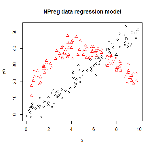
Below you can see example of such model from flexmix library (Leisch, 2004; Grun and Leisch, 2008) vignette fitting mixture of two regression models to made-up data.

library("flexmix")
data("NPreg")
m1 <- flexmix(yn ~ x + I(x^2), data = NPreg, k = 2)
summary(m1)
## 
## Call:
## flexmix(formula = yn ~ x + I(x^2), data = NPreg, k = 2)
## 
##        prior size post>0 ratio
## Comp.1 0.506  100    141 0.709
## Comp.2 0.494  100    145 0.690
## 
## 'log Lik.' -642.5452 (df=9)
## AIC: 1303.09   BIC: 1332.775 
parameters(m1, component = 1)
##                      Comp.1
## coef.(Intercept) 14.7171662
## coef.x            9.8458171
## coef.I(x^2)      -0.9682602
## sigma             3.4808332
parameters(m1, component = 2)
##                       Comp.2
## coef.(Intercept) -0.20910955
## coef.x            4.81646040
## coef.I(x^2)       0.03629501
## sigma             3.47505076

It is visualized on the following plots (points shapes are the true classes, colors are the classifications).

References and additional resources

For further details you can check the following books and papers:

Wedel, M. and DeSarbo, W.S. (1995). A Mixture Likelihood Approach for Generalized Linear Models. Journal of Classification , 12, 21–55.

Wedel, M. and Kamakura, W.A. (2001). Market Segmentation – Conceptual and Methodological Foundations. Kluwer Academic Publishers.

Leisch, F. (2004). Flexmix: A general framework for finite mixture models and latent glass regression in R. Journal of Statistical Software, 11(8), 1-18.

Grun, B. and Leisch, F. (2008). FlexMix version 2: finite mixtures with concomitant variables and varying and constant parameters. Journal of Statistical Software, 28(1), 1-35.

McLachlan, G. and Peel, D. (2000). Finite Mixture Models. John Wiley & Sons.

Dayton, C.M. and Macready, G.B. (1988). Concomitant-Variable Latent-Class Models. Journal of the American Statistical Association, 83(401), 173-178.

Linzer, D.A. and Lewis, J.B. (2011). poLCA: An R package for polytomous variable latent class analysis. Journal of Statistical Software, 42(10), 1-29.

McCutcheon, A.L. (1987). Latent Class Analysis. Sage.

Hagenaars J.A. and McCutcheon, A.L. (2009). Applied Latent Class Analysis. Cambridge University Press.

Vermunt, J.K., and Magidson, J. (2003). Latent class models for classification. Computational Statistics & Data Analysis, 41(3), 531-537.

Grün, B. and Leisch, F. (2007). Applications of finite mixtures of regression models. flexmix package vignette.

Grün, B., & Leisch, F. (2007). Fitting finite mixtures of generalized linear regressions in R. Computational Statistics & Data Analysis, 51(11), 5247-5252.

Answer 2

Multi-Task Learning MLT allows different types of loss-functions ( for example, least-square for regression and logistic or Hinge loss for classification) to be optimized simultaneously. the components of this heterogeneous loss function can be weighted to control/ distinguish the main task from the secondary one. if the two tasks do not have the same learning difficulties and convergence rates; a stop criterion has to be introduced for the simpler task to avoid overfitting. a 3rd component can also be introduced to the loss-function to ensure smoothness of the whole learning process. the heterogeneous loss function may look like that (a case for regression and classification):

notice the applied weight to the logistic loss function, and the last regularization term for eights penalization

Now if we want to implement this with Pytorch, we have to split the output and run it through different criteria (again MSE for regression and logistic loss for classification)

let yhat the inintial output of the model that is splited into yhat_1 and yhat_2 such :
yhat = concat(yhat_1, yhat_2)

the same for y the ground truth. in the learning step the model should be optimized as follow:

criterion1 = nn.MSELoss()
criterion2 = nn.BCELoss()
loss1 = criterion1(yhat_1, y1)
loss2 = criterion1(yhat_2, y2)
loss = loss1 + lambda*loss2
loss.backward()