What is the explanation of the difference caused by the order of variables in anova for the concrete example in R?

Question

I wonder the real reason behind the difference in results of the two anovas that use the same covariates. However, the results are different.

library(PASWR2)
head(HSWRESTLER); tail(HSWRESTLER)
#  age    ht    wt abs triceps subscap hwfat tanfat skfat
# 1  18 65.75 133.6   8       6    10.5 10.71   11.9  9.80
# 2  15 65.50 129.0  10       8     9.0  8.53   10.0 10.56
# ...
# 77  15 68 153.8  13       7      11 10.07   16.7 11.77
# 78  15 66 258.6  45      37      43 33.75   34.5 38.93

mod1.HSW <- lm(hwfat ~ abs + triceps + subscap, data = HSWRESTLER)
anova(mod1.HSW)
# Analysis of Variance Table
# Response: hwfat              
#            Df Sum Sq Mean Sq F value    Pr(>F)     
# abs        1 5072.8  5072.8 535.858 < 2.2e-16 ***    
# triceps    1  242.2   242.2  25.581 2.984e-06 ***    
# subscap    1    2.2     2.2   0.237    0.6278        
# Residuals 74  700.5     9.5   
# ---
# Signif. codes:  0 ‘***’ 0.001 ‘**’ 0.01 ‘*’ 0.05 ‘.’ 0.1 ‘ ’ 1

mod2.HSW <- lm(hwfat ~ subscap + triceps + abs, data = HSWRESTLER)
anova(mod2.HSW) # ANOVA
# Analysis of Variance Table
# Response: hwfat
#           Df Sum Sq Mean Sq F value    Pr(>F)    
# subscap    1 4939.0  4939.0 521.720 < 2.2e-16 ***
# triceps    1  204.6   204.6  21.616 1.422e-05 ***
# abs        1  173.6   173.6  18.341 5.473e-05 ***
# Residuals 74  700.5     9.5                      
# ---
# Signif. codes:  0 ‘***’ 0.001 ‘**’ 0.01 ‘*’ 0.05 ‘.’ 0.1 ‘ ’ 1

?anova help file is not explanatory enough about what is going on. The similar SOF questions does not handle the situation with a concrete example like this. The variables in the regressions seem to be continuous variables (covariates). It seems the variable order is important. But, what does that order mean? What can be inferred from the above two anovas? Any idea?

Answer 1

When you call anova on an lm model fit, under the hood you are really using ?anova.lm, which according to the documentation "gives a sequential analysis of variance table for that fit." This is a type I ANOVA, where order of the variables matter.The term abs in your second example only represents the unique portion of the regression explained given the previous two variables.

You can perform type II ANOVA using drop1(). Here order doesn't matter, thus each main effect can be understood as the individual contribution of that predictor:

> drop1(mod1.HSW)
#Single term deletions
#
#Model:
#hwfat ~ abs + triceps + subscap
#        Df Sum of Sq    RSS    AIC
#<none>               700.54 179.22
#abs      1   173.629 874.17 194.49
#triceps  1   111.837 812.38 188.77
#subscap  1     2.244 702.78 177.47

> drop1(mod2.HSW)
#Single term deletions
#
#Model:
#hwfat ~ subscap + triceps + abs
#        Df Sum of Sq    RSS    AIC
#<none>               700.54 179.22
#subscap  1     2.244 702.78 177.47
#triceps  1   111.837 812.38 188.77
#abs      1   173.629 874.17 194.49

Answer 2

I like to understand linear regression in terms of its computation. A linear model is computed by QR factorization, giving a number of "effects" on the rotated plane. You can refer to What is the “effects” returned by aov and lm? for details.

"Effects" is the key for generating ANOVA table:

e1 <- mod1.HSW$effects[2:4]  ## we also exclude "Intercept"
#       abs     triceps     subscap 
# 71.223840   15.561899   -1.497877 

e2 <- mod2.HSW$effects[1:4]  ## we also exclude "Intercept"
#  subscap     triceps         abs 
# 70.27797    14.30491    13.17682 

Note, effects are already different, due to order of terms. Two models are equivalent, so they have the same residual variance:

d <- with(mod1.HSW, c(crossprod(residual)) / df.residual)
# [1] 9.466757

ANOVA table and F-statistic can be compute as:

cbind("explained-variance" = e1 ^ 2, "F-statistic" = e1 ^ 2 / d)

#            explained-variance  F-statistic
#abs                5072.835390  535.8577814
#triceps             242.172704   25.5813797
#subscap               2.243634    0.2370014

cbind("explained-variance" = e2 ^ 2, "F-statistic" = e2 ^ 2 / d)

#            explained-variance F-statistic
#subscap              4938.9927   521.71960
#triceps               204.6305    21.61569
#abs                   173.6286    18.34087

Have a comparison with anova(mod1.HSW) and anova(mod2.HSW) yourself.

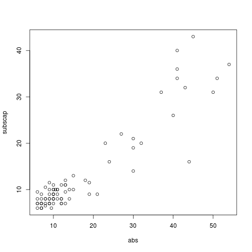
To this stage, you should realize that the difference in "effects" explains why ANOVA table is different. lm performs non-pivoted QR factorization, hence is sensitive to term orders. QR factorization for a matrix X is like a "Gram-Schmidt" process. If you have 2 columns linearly correlated, then reversing these two columns will make QR factorization different.

Now have a look at your data:

with(HSWRESTLER, plot(abs, subscap))

Isn't this a linear relationship?