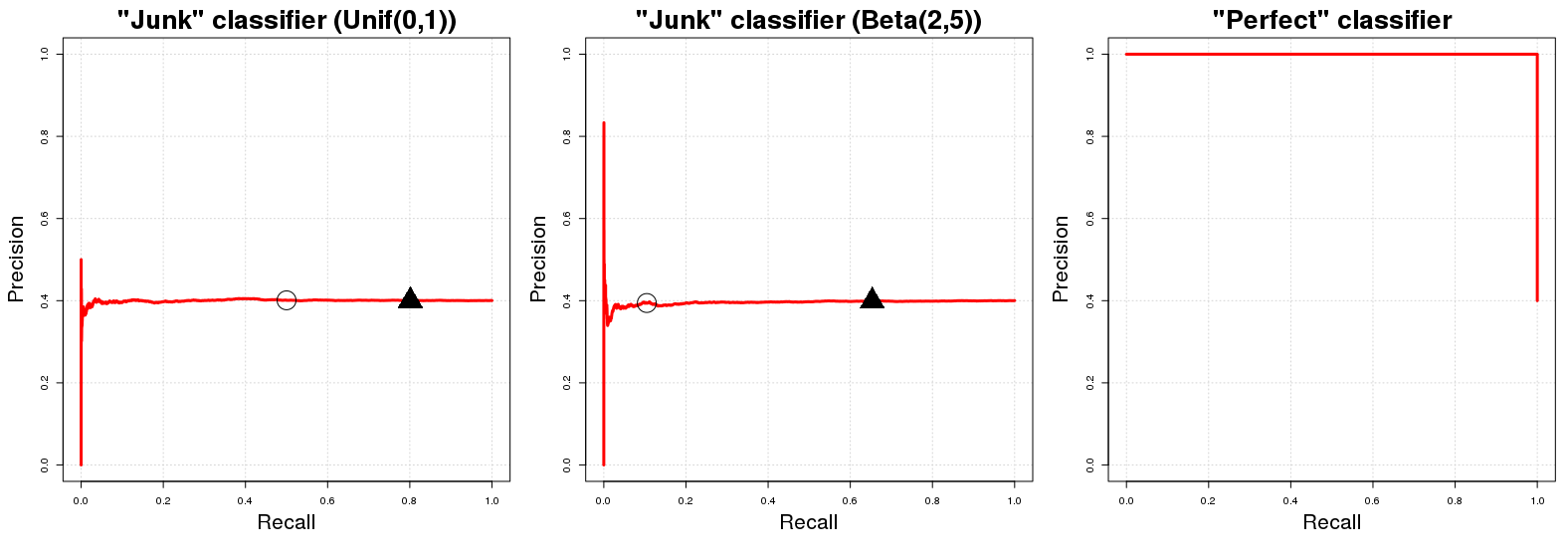
The "baseline curve" in a PR curve plot is a horizontal line with height equal to the number of positive examples $P$ over the total number of
training data $N$, ie. the proportion of positive examples in our data ($\frac{P}{N}$).
OK, why is this the case though? Let's assume we have a "junk classifier" $C_J$. $C_J$ returns a random probability $p_i$ to the $i$-th sample instance $y_i$ to be in class $A$. For convenience, say $p_i \sim U[0,1]$.
The direct implication of this random class assignment is that $C_J$ will have (expected) precision equal to the proportion of positive examples in our data. It is only natural; any totally random sub-sample of our data will have $E\{\frac{P}{N}\}$ correctly classified examples. This will be true for any probability threshold $q$ we might use as a decision boundary for the probabilities of class membership returned by $C_J$. ($q$ denotes a value in $[0,1]$ where probability values greater or equal to $q$ are classified in class $A$.)
On the other hand the recall performance of $C_J$ is (in expectation) equal to $q$ if $p_i \sim U[0,1]$. At any given threshold $q$ we will pick (approximately) $(100(1-q))\%$ of our total data which subsequently will contain (approximately) $(100(1-q))\%$ of the total number of instances of class $A$ in the sample.
Hence the horizontal line we mentioned at the beginning! For every recall value ($x$ values in PR graph) the corresponding precision value ($y$ values in the PR graph) is equal to $\frac{P}{N}$.
A quick side-note: The threshold $q$ is not generally equal to 1 minus the expected recall. This happens in the case of a $C_J$ mentioned above only because of the random uniform distribution of $C_J$'s results; for a different distribution (eg. $ p_i \sim B(2,5)$) this approximate identity relation between $q$ and recall does not hold; $U[0,1]$ was used because it is the easiest to understand and mentally visualise. For a different random distribution in $[0,1]$ the PR profile of $C_J$ will not change though. Just the placement of P-R values for given $q$ values will change.
Now regarding a perfect classifier $C_P$, one would mean a classifier that returns probability $1$ to sample instance $y_i$ being of class $A$ if $y_i$ is indeed in class $A$ and additionally $C_P$ returns probability $0$ if $y_i$ is not a member of class $A$. This implies that for any threshold $q$ we will have $100\%$ precision (ie. in graph-terms we get a line starting at precision $100\%$). The only point we do not get $100\%$ precision is at $q = 0$. For $q=0$, the precision falls to the proportion of positive examples in our data ($\frac{P}{N}$) as (insanely?) we classify even points with $0$ probability of being of class $A$ as being in class $A$. The PR graph of $C_P$ has just two possible values for its precision, $1$ and $\frac{P}{N}$.
OK and some R code to see this first handed with an example where the positive values correspond to $40\%$ of our sample. Notice that we do a "soft-assignment" of class category in the sense that the probability value associated with each point quantifies to our confidence that this point is of class $A$.
  rm(list= ls())
  library(PRROC)
  N = 40000
  set.seed(444)
  propOfPos = 0.40
  trueLabels = rbinom(N,1,propOfPos)
  randomProbsB = rbeta(n = N, 2, 5)
  randomProbsU = runif(n = N)

  # Junk classifier with beta distribution random results
  pr1B <- pr.curve(scores.class0 = randomProbsB[trueLabels == 1],
                   scores.class1 = randomProbsB[trueLabels == 0], curve = TRUE)
  # Junk classifier with uniformly distribution random results
  pr1U <- pr.curve(scores.class0 = randomProbsU[trueLabels == 1],
                   scores.class1 = randomProbsU[trueLabels == 0], curve = TRUE)
  # Perfect classifier with prob. 1 for positives and prob. 0 for negatives.
  pr2 <- pr.curve(scores.class0 = rep(1, times= N*propOfPos),
                  scores.class1 = rep(0, times = N*(1-propOfPos)), curve = TRUE)

  par(mfrow=c(1,3))
  plot(pr1U, main ='"Junk" classifier (Unif(0,1))', auc.main= FALSE,
       legend=FALSE, col='red', panel.first= grid(), cex.main = 1.5);
  pcord = pr1U$curve[ which.min( abs(pr1U$curve[,3]- 0.50)),c(1,2)];
  points( pcord[1], pcord[2], col='black', cex= 2, pch = 1)
  pcord = pr1U$curve[ which.min( abs(pr1U$curve[,3]- 0.20)),c(1,2)];
  points( pcord[1], pcord[2], col='black', cex= 2, pch = 17)
  plot(pr1B, main ='"Junk" classifier (Beta(2,5))', auc.main= FALSE,
       legend=FALSE, col='red', panel.first= grid(), cex.main = 1.5);
  pcord = pr1B$curve[ which.min( abs(pr1B$curve[,3]- 0.50)),c(1,2)];
  points( pcord[1], pcord[2], col='black', cex= 2, pch = 1)
  pcord = pr1B$curve[ which.min( abs(pr1B$curve[,3]- 0.20)),c(1,2)];
  points( pcord[1], pcord[2], col='black', cex= 2, pch = 17)
  plot(pr2, main = '"Perfect" classifier', auc.main= FALSE,
       legend=FALSE, col='red', panel.first= grid(), cex.main = 1.5);

where the black circles and triangles denote $q =0.50$ and $q=0.20$ respectively in the first two plots. We immediately see that the "junk" classifiers quickly go to precision equal to $\frac{P}{N}$; similarly the perfect classifier has precision $1$ across all recall variables. Unsurprisingly, the AUCPR for the "junk" classifier is equal to the proportion of positive example in our sample ($\approx 0.40$) and the AUCPR for the "perfect classifier" is approximately equal to $1$.
Realistically the PR graph of a perfect classifier is a bit useless because one cannot have $0$ recall ever (we never predict only the negative class); we just start plotting the line from the upper left corner as a matter of convention. Strictly speaking it should just show two points but this would make a horrible curve. :D
For the record, there are already have been some very good answer in CV regarding the utility of PR curves: here, here and here. Just reading through them carefully should offer a good general understand about PR curves.

