0
$\begingroup$

I tried searching for this question on stats stack exchange and found Implementing linear regression with standardization but the answer was a little difficult to follow. I'm reading "Bayesian Analysis with Python" by Osvaldo Martin (great read btw) and in his hierarchical linear models section he often mean-centers the data and the reverses it. Can somebody please explain this process to me and how to rearrange the values to visualize the reversal after mean-centering? The line that is confusing me is alpha = pm.Deterministic("alpha", alpha_tmp - pm.math.dot(beta, X_mean)) why does subtracting the dot product of the betas and the mean from the alphas reverse the mean centering? I feel like I'm missing something very simple.

The author implements it in Python 3.5 using a module that is up and coming called pymc3. Here is the code excerpt below:

alpha_tmp is the alpha when X is mean centered. The formula that is being used is:

$$\mu = \alpha + \beta_1*x_1 + \beta_2*x_2$$

import pymc3 as pm
import numpy as np

# Multiple Linear Regression
# pg. 132
np.random.seed(314)
N = 100
alpha_real = 2.5
beta_real = [0.9, 1.5]
eps_real = np.random.normal(loc=0, scale=0.5, size=N)

X = np.array([np.random.normal(i,j, N) for i,j in zip([10,2],[1,1.5])])

X_mean = X.mean(axis=1, keepdims=True)
X_centered = X - X_mean
y = alpha_real + np.dot(beta_real, X) + eps_real

with pm.Model() as model_mlr:
    alpha_tmp = pm.Normal("alpha_tmp", mu=0, sd=10)
    beta = pm.Normal("beta", mu=0, sd=1, shape=2)
    epsilon = pm.HalfCauchy("epsilon", 5)

    mu = alpha_tmp + pm.math.dot(beta, X_centered)

    alpha = pm.Deterministic("alpha", alpha_tmp - pm.math.dot(beta, X_mean))

    y_pred = pm.Normal("y_pred", mu=mu, sd=epsilon, observed=y)

    start = pm.find_MAP()
    step = pm.NUTS(scaling-start)
    trace_mlr = pm.sample(5000, step=step, start=start)

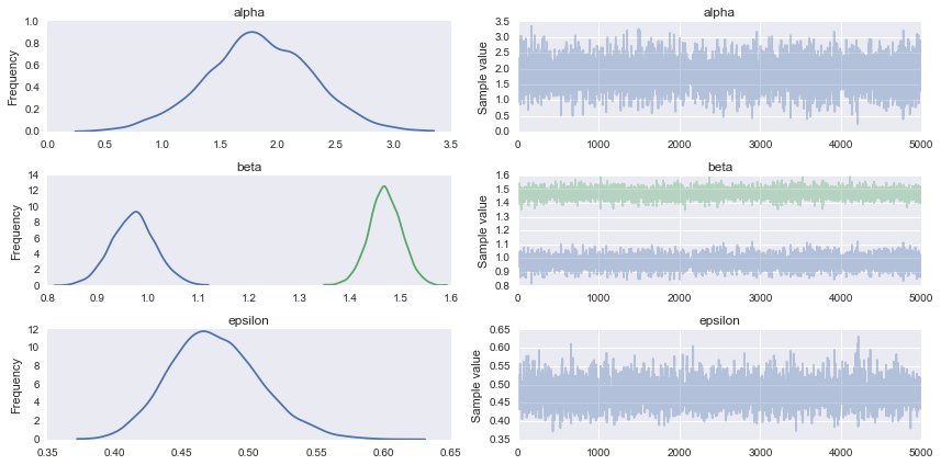
varnames = ["alpha", "beta", "epsilon"]
pm.traceplot(trace_mlr, varnames)

# Below is output of stderr
Optimization terminated successfully.
         Current function value: 74.986175
         Iterations: 23
         Function evaluations: 31
         Gradient evaluations: 31
100%|██████████| 5000/5000 [00:13<00:00, 380.52it/s]

enter image description here

$\endgroup$

2 Answers 2

1
$\begingroup$

The answer by John Kruschke is the right one. And is also explained on page 102 of "Bayesian Analysis with Python" (BAP). Since the explanation in BAP is very brief, and probably not clear enough (sorry about that!) I will give here a little bit more detail:

We get $x'$, the centered version of $x$ by doing:

$$x' = x - \bar x$$

Then we can write the linear model as:

$$y = \alpha' + \beta' x' + \epsilon$$

if we replace $x'$ with $x - \bar x$, we get:

$$y = \alpha' + \beta' (x - \bar x) + \epsilon$$

reordering we get:

$$y = \alpha' - \beta' \bar x + \beta' x + \epsilon$$

Notice that this last equation is equivalent to

$$y = \alpha + \beta x + \epsilon$$

where:

$$\alpha = \alpha' - \beta' x$$

and

$$\beta = \beta' $$

$\endgroup$
4
  • $\begingroup$ Thanks! That makes a lot of sense. I didn't know the the beta's are conserved between normalized and unnormalized models. I also don't have the Doing Bayesian Data Analysis book but I heard it's a great resource. $\endgroup$
    – O.rka
    Commented Dec 28, 2016 at 6:13
  • 1
    $\begingroup$ Notice that we are centering the data, not standardizing/normalizing it. The range of the data is the same. That's why the betas are not changing. $\endgroup$ Commented Dec 28, 2016 at 13:29
  • $\begingroup$ Yes, thank you for pointing that out. I tend to use the term normalization loosely. If one were to divide by the standard deviation to normalize this, you would be able to reverse it right? I'm a little confused going from $y = \alpha' + \beta'\bar x + \beta 'x + \epsilon$ to $\alpha = \alpha' - \beta x$ when I set $ \alpha' + \beta'\bar x + \beta'x + \epsilon = \alpha + \beta x + \epsilon$ it simplifies to $\alpha' - \beta'\bar x = x(\beta - \beta') + \alpha$ $\endgroup$
    – O.rka
    Commented Dec 28, 2016 at 18:29
  • 1
    $\begingroup$ If you divide by the standard deviation you would be able to reverse it. Notice that in many setting you don't need/want to reverse the transformations. You just need to be careful when interpreting the parameters. In many problems interpreting the parameters in the normalized space could in fact be easier or more useful. $\endgroup$ Commented Jan 3, 2017 at 14:07
0
$\begingroup$

It's explained on p. 485 of Doing Bayesian Data Analysis Second Edition.

Just start with the predictiin equation for mean centered parameters, substitute the mean centered variables, and reexpress in terms of the original variables.

$\endgroup$

Your Answer

By clicking “Post Your Answer”, you agree to our terms of service and acknowledge you have read our privacy policy.

Not the answer you're looking for? Browse other questions tagged or ask your own question.