20
$\begingroup$

When running an ANOVA we are told that certain assumptions of the test must be present for it to be applicable to the data. I never understood the reason as to why the following assumptions were necessary for the test to function:

  1. The variance of your dependent variable (residuals) should be equal in each cell of the design

  2. Your dependent variable (residuals) should be approximately normally distributed for each cell of the design

I understand that there is a bit of a grey area as to if these assumptions need to be met, but for the sake of argument, if these assumptions were utterly not met in a given data set, what would be the issue with using an ANOVA?

$\endgroup$
1
  • $\begingroup$ what is the goal of your study ? $\endgroup$
    – user10619
    Commented Jan 13, 2017 at 1:44

3 Answers 3

12
$\begingroup$

The assumptions matter insofar as they affect the properties of the hypothesis tests (and intervals) you might use whose distributional properties under the null are calculated relying on those assumptions.

In particular, for hypothesis tests, the things we might care about are how far the true significance level might be from what we want it to be, and whether power against alternatives of interest is good.

In relation to the assumptions you ask about:

1. Equality of variance

The variance of your dependent variable (residuals) should be equal in each cell of the design

This can certainly impact the significance level, at least when sample sizes are unequal.

(Edit:) An ANOVA F-statistic is the ratio of two estimates of variance (the partitioning and comparison of variances is why it's called analysis of variance). The denominator is an estimate of the supposedly-common-to-all-cells error variance (calculated from residuals), while the numerator, based on variation in the group means, will have two components, one from variation in the population means and one due to the error variance. If the null is true, the two variances that are being estimated will be the same (two estimates of the common error variance); this common but unknown value cancels out (because we took a ratio), leaving an F-statistic that only depends on the distributions of the errors (which under the assumptions we can show has an F distribution. (Similar comments apply to the t-test I used for illustration.)

[There's a little bit more detail on some of that information in my answer here]

However, here the two population variances differ across the two differently-sized samples. Consider the denominator (of the F-statistic in ANOVA and of the t-statistic in a t-test) - it is composed of two different variance estimates, not one, so it will not have the "right" distribution (a scaled chi-square for the F and its square root in the case of a t - both the shape and the scale are issues).

As a result, the F-statistic or the t-statistic will no longer have the F- or t-distribution, but the manner in which it is affected is different depending on whether the large or the smaller sample was drawn from the population with the larger variance. This in turn affects the distribution of p-values.

Under the null (i.e. when the population means are equal), the distribution of p-values should be uniformly distributed. However, if the variances and the sample sizes are unequal but the means are equal (so we don't want to reject the null), the p-values are not uniformly distributed. I did a small simulation to show you what happens. In this case, I used only 2 groups so ANOVA is equivalent to a two-sample t-test with the equal variance assumption. So I simulated samples from two normal distributions one with standard deviation ten times as large as the other, but equal means.

For the left side plot, the larger (population) standard deviation was for n=5 and the smaller standard deviation was for n=30. For the right side plot the larger standard deviation went with n=30 and the smaller with n=5. I simulated each one 10000 times and found the p-value each time. In each case you want the histogram to be completely flat (rectangular), since this means all tests conducted at some significance level $\alpha$ with actually get that type I error rate. In particular it's most important that the leftmost parts of the histogram to stay close to the grey line:
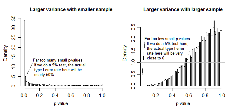
Histograms of p-values for simulated samples

As we see, the left side plot (larger variance in the smaller sample) the p-values tend to be very small -- we would reject the null hypothesis very often (nearly half the time in this example) even though the null is true. That is, our significance levels are much larger than we asked for. In the right hand side plot we see the p-values are mostly large (and so our significance level is much smaller than we asked for) -- in fact not once in ten thousand simulations did we reject at the 5% level (the smallest p-value here was 0.055). [This may not sound like such a bad thing, until we remember that we will also have very low power to go with our very low significance level.]

That's quite a consequence. This is why it's a good idea to use a Welch-Satterthwaite type t-test or ANOVA when we don't have a good reason to assume that the variances will be close to equal -- by comparison it's barely affected in these situations (I simulated this case as well; the two distributions of simulated p-values - which I have not shown here - came out quite close to flat).

2. Conditional distribution of the response (DV)

Your dependent variable (residuals) should be approximately normally distributed for each cell of the design

This is somewhat less directly critical - for moderate deviations from normality, the significance level is so not much affected in larger samples (though the power can be!).

Here's one example, where the values are exponentially distributed (with identical distributions and sample sizes), where we can see this significance level issue being substantial at small $n$ but reducing with large $n$.
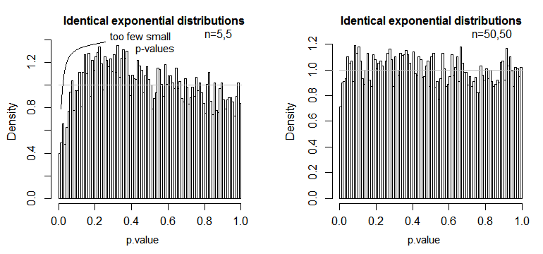
histograms of p-values when H0 is true but the distributions in each group are exponential

We see that at n=5 there are substantially too few small p-values (the significance level for a 5% test would be about half what it should be), but at n=50 the problem is reduced -- for a 5% test in this case the true significance level is about 4.5%.

So we might be tempted to say "well, that's fine, if n is big enough to get the significance level to be pretty close", but we may also be throwing a way a good deal of power. In particular, it's known that the asymptotic relative efficiency of the t-test relative to widely used alternatives can go to 0. This means that better test choices can get the same power with a vanishingly small fraction of the sample size required to get it with the t-test. You don't need anything out of the ordinary to be going on to need more than say twice as much data to have the same power with the t as you would need with an alternative test - moderately heavier-than normal tails in the population distribution and moderately large samples can be enough to do it.

(Other choices of distribution may make the significance level higher than it should be, or substantially lower than we saw here.)

$\endgroup$
3
  • $\begingroup$ Thanks Glen for the detailed response. I am curious as to why the errors that you have described would occur if assumptions were not met In terms of equality of variance, am I correct in taking from your writing the following?: The issue arising from having a smaller sample size group having the larger variance is (as well as the number of data points being small in general i.e. n = 5) that the larger variance observed in the smaller sample is being calculated as representative of the variance at the population level . $\endgroup$ Commented Jan 13, 2017 at 21:41
  • $\begingroup$ (part 2) Its essentially an unfair comparison between a representative sample and an under representative sample (relatively speaking) which can lead to a type 1 error due to how ANOVA is processed. $\endgroup$ Commented Jan 13, 2017 at 21:41
  • $\begingroup$ @Paper I don't think that's the issue here. It is not the representativeness of the sample variance in the smaller sample (e.g. if both samples were equally small, you'd have twice the problem with representativeness, but this issue would be absent). I've added a few paragraphs to my answer to explain how the issue arises in more detail. $\endgroup$
    – Glen_b
    Commented Jan 13, 2017 at 22:37
10
$\begingroup$

In a nutshell, ANOVA is adding, squaring and averaging residuals. Residuals tell you how well your model fits the data. For this example, I used the PlantGrowth dataset in R:

Results from an experiment to compare yields (as measured by dried weight of plants) obtained under a control and two different treatment conditions.

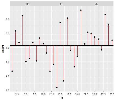
This first plot shows you the grand mean across all three treatment levels:

enter image description here

The red lines are the residuals. Now by squaring and adding the length of those individual lines, you will get a value that tells you how well the mean (our model) describes the data. A small number, tells you the mean describes your data points well, a bigger number tells you the mean describes your data not so well. This number is called the Total Sums of Squares:

$SS_{total}=\sum(x_i-\bar{x}_{grand})^2$, where $x_{i}$ represents the individual data point and $\bar{x}_{grand}$ the grand mean across the dataset.

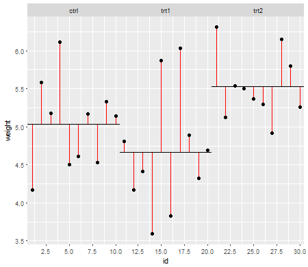
Now you do the same thing for the residuals in your treatment (Residual Sums of Squares, which is also known as the noise in the treatment levels):

enter image description here

And the formula:

$SS_{residuals}=\sum(x_{ik}-\bar{x}_{k})^2$, where $x_{ik}$ are the individual data points $i$ in the $k$ number of levels and $\bar{x}_{k}$ the mean across the treatment levels.

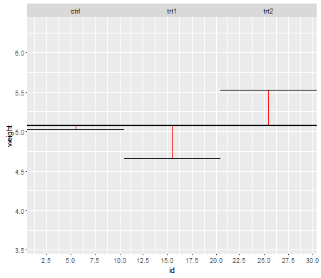
Lastly, we need to determine the signal in the data, which is known as the Model Sums of Squares, which will later be used to calculate whether the treatment means are any different from the grand mean:

enter image description here

And the formula:

$SS_{model}=\sum n_{k}(\bar{x}_k-\bar{x}_{grand})^2$, where $n_{k}$ is the sample size $n$ in your $k$ number of levels, and $\bar{x}_k$ as well as $\bar{x}_{grand}$ the mean within and across the treatment levels, respectively.

Now the disadvantage with the sums of squares is that they get bigger as the sample size increase. To express those sums of squares relative to the number of observation in the data set, you divide them by their degrees of freedom turning them into variances. So after squaring and adding your data points you are now averaging them using their degrees of freedom:

$df_{total}=(n-1)$

$df_{residual}=(n-k)$

$df_{model}=(k-1)$

where $n$ is the total number of observations and $k$ the number of treatment levels.

This results in the Model Mean Square and the Residual Mean Square (both are variances), or the signal to noise ratio, which is known as the F-value:

$MS_{model}=\frac{SS_{model}}{df_{model}}$

$MS_{residual}=\frac{SS_{residual}}{df_{residual}}$

$F=\frac{MS_{model}}{MS_{residual}}$

The F-value describes the signal to noise ratio, or whether the treatment means are any different from the grand mean. The F-value is now used to calculate p-values and those will decide whether at least one of the treatment means will be significantly different from the grand mean or not.

Now I hope you can see that the assumptions are based on calculations with residuals and why they are important. Since we adding, squaring and averaging residuals, we should make sure that before we are doing this, the data in those treatment groups behaves similar, or else the F-value may be biased to some degree and inferences drawn from this F-value may not be valid.

Edit: I added two paragraphs to address the OP's question 2 and 1 more specifically.

Normality assumption: The mean (or expected value) is often used in statistics to describe the center of a distribution, however it is not very robust and easily influenced by outliers. The mean is the simplest model we can fit to the data. Since in ANOVA we are using the mean to calculate the residuals and the sums of squares (see formulae above), the data should be roughly normally distributed (normality assumption). If this is not the case, the mean may not be the appropriate model for the data since it wouldn’t give us a correct location of the center of the sample distribution. Instead once could use the median for example (see non parametric testing procedures).

Homogeneity of variance assumption: Later when we calculate the mean squares (model and residual), we are pooling the individual sums of squares from the treatment levels and averaging them (see formulae above). By pooling and averaging we are losing the information of the individual treatment level variances and their contribution to the mean squares. Therefore, we should have roughly the same variance among all treatment levels so that the contribution to the mean squares is similar. If the variances between those treatment levels were different, then the resulting mean squares and F-value would be biased and will influence the calculation of the p-values making inferences drawn from these p-values questionable (see also @whuber 's comment and @Glen_b 's answer).

This is how I see it for myself. It may not be 100% accurate (I am not a statistician) but it helps me understanding why satisfying the assumptions for ANOVA is important.

$\endgroup$
4
  • 1
    $\begingroup$ Your account is good, but you stopped just short of answering the question! The $F$ statistic is a useful description of the ANOVA no matter what. The homoscedasticity and normality assumptions are needed so that the $F$ statistic will actually have an $F$ ratio distribution; moreover, relatively small violations of either assumption tend to cause the $F$ statistic's distribution to depart noticeably from the $F$ ratio distribution, casting doubt on any p-values computed from it. That is why other answers, such as by @Glen_b, focus on this distribution. $\endgroup$
    – whuber
    Commented Jan 13, 2017 at 18:15
  • $\begingroup$ @whuber I appreciate your comment, it helps me learn. I will have to let this sink in and spend some time looking at the $F$ ratio vs the $F$ statistic distributions and how they influence the calculations of the p-values. $\endgroup$
    – Stefan
    Commented Jan 13, 2017 at 18:23
  • $\begingroup$ Thanks Stefan. I want to see if I am understanding you correctly. ANOVA essentially creates a grand mean out of all the data points of the set and compares how far away each group differs from this grand mean to understand if their is a statistically significant difference among them. If the discussed assumptions are not met, the grand mean is not very reflective of the groups being compared and it leads to a difficulty of comparison $\endgroup$ Commented Jan 13, 2017 at 20:04
  • $\begingroup$ @PaperRockBazooka In an ANOVA you are comparing signal to noise. If you cannot detect a signal, i.e. the effect of your treatment on the outcome, you might as well take the grand mean as the model to describe the data. We are using the difference of the data points to the grand mean ($SS_{total}$), the difference of the data points to the treatment means ($SS_{residual}$), and the difference of the treatment means to the grand mean ($SS_{model}$) to determine the signal to noise ratio. Try to calculate a simple One-Way ANOVA by hand. That helped me to understand it better. $\endgroup$
    – Stefan
    Commented Jan 13, 2017 at 22:16
0
$\begingroup$

ANOVA it's just a method, it calculates the F-test from your samples and it compares it to the F-distribution. You need some assumptions to decide what you want to compare and to calculate the p-values.

If you don't meet that assumptions you could calculate other things but it won't be an ANOVA.

The most useful distribution is the normal one (because of the CLT), that's why it's the most commonly used. If your data it's not normally distributed you need at least to know what's its distribution in order to calculate something.

Homoscedasticity is a common assumption also in regression analysis, it just makes things easier. We need some assumptions to start with.

If you don't have homoscedasticity you can try transform your data to achieve it.

The ANOVA F-test is known to be nearly optimal in the sense of minimizing false negative errors for a fixed rate of false positive errors

$\endgroup$
1
  • 1
    $\begingroup$ "ANOVA" refers to the process of decomposing sums of squares into interpretable components. Regardless of the distributional assumptions, then, an ANOVA is an ANOVA. $\endgroup$
    – whuber
    Commented Jan 13, 2017 at 18:18

Your Answer

By clicking “Post Your Answer”, you agree to our terms of service and acknowledge you have read our privacy policy.

Not the answer you're looking for? Browse other questions tagged or ask your own question.