1
$\begingroup$

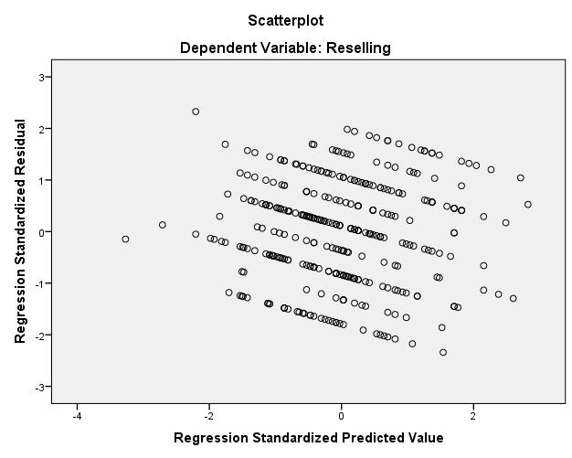
The following is the residuals vs predicted scatter plot for a regression model with two IVs. enter image description here

Initially, I thought it was evidence of heteroskedasticity. But, I reasoned that although there is a visible pattern in the plot, the variance across different levels of predicted values is same.

To clear my doubts, I saved the standardized residual and predicted values and ran a bi-variate correlation test. The correlation is zero, as expected. I am, nevertheless, intrigued by this observation. Any idea why I might have obtained this pattern?

PS:- My dependent variable is a sum of two likert-type items (Response scale: 1-5). So, it's theoretical range is 2-10 and it has no absolute zero value.

$\endgroup$
8
  • 3
    $\begingroup$ What aspect of the pattern are you intrigued by? The variables are not truly continuous, so you get stripes in the plot. It's also likely that you have points on top of each other so you can't see how many points are in one place. Can you jitter, or add sunflowers? $\endgroup$ Commented Jan 13, 2017 at 5:46
  • $\begingroup$ I@JeremyMiles You make some good points but the negative slope is striking to me. Maybe there is another predictor that is not accounted for and so it appears in the residuals. $\endgroup$ Commented Jan 13, 2017 at 5:58
  • 1
    $\begingroup$ Often asked here, e.g stats.stackexchange.com/questions/188529/…. Think back to residual $=$ observed $-$ fitted, implying that in this graph with fitted or predicted on horizontal axis each distinct value of the observed lies on a particular line with negative slope (standardization may affect the slope, but not the existence of a collective pattern). Plot not a point but the numeric value of your response and you'll see the pattern. An inevitable artefact that really should not seem surprising. $\endgroup$
    – Nick Cox
    Commented Jan 13, 2017 at 7:33
  • 1
    $\begingroup$ @Glen_b and I have answered this more than once, but for the moment I can't find a good duplicate. $\endgroup$
    – Nick Cox
    Commented Jan 13, 2017 at 7:38
  • 1
    $\begingroup$ Note that this isn't a visual illusion; nor do other predictors need to be invoked. Other predictors would change fitted and residual but the lines would remain. $\endgroup$
    – Nick Cox
    Commented Jan 13, 2017 at 10:21

1 Answer 1

2
$\begingroup$

Here is an example set-up with observed response just 2(1)10 as reported.

The Stata code should seem fairly transparent even to those who have never used it. gen means generate.

clear 
set obs 500 
set seed 2803 

gen y = round(rnormal(6, 1.5), 1) 
gen x1 = rnormal()
gen x2 = rnormal() 

regress y x1 x2 
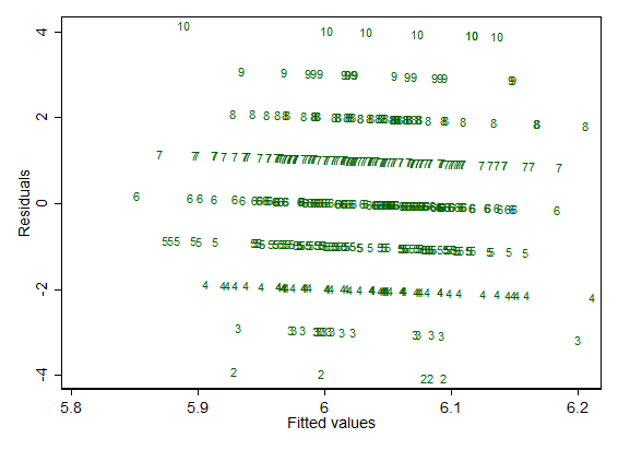
rvfplot , mla(y) mlabpos(0) ms(none) 
enter image description here

I'm just regressing the response against Gaussian noise in this example, but the features noticeable on this plot are generic.

For each distinct observed response, there is a line

residual $=$ observed $-$ fitted

So, for observed $= 7$, all those points lie on the line

residual $= 7 -$ fitted

and the slope with fitted is negative (here, where there is no standardization or other adjustment, it is exactly $-1$).

That's always true. Naturally at one extreme if each value of the response is (literally) unique, each line is represented by just a single point and won't be discernible as such. But whenever there are just a few distinct values, as here, the lines will be discernible.

Plotting the numeric values of the response is not standard but surely a useful option to make clear what is happening. If your favourite software won't allow it, you need to change to a new favourite.

Incidentally, I prefer to see the actual values of residual and fitted on these graphs.

Not the question, but with small discrete responses it's worth keeping tracking of whether the model is predicting impossible values. Plain linear regression may be a poor idea for such data.
$\endgroup$
2
  • $\begingroup$ Thanks for the response. If I understand correctly, this plot is expected in any model where the DV is a non-continuous scale variable. This, perhaps, can be linked to the much debated question of whether scale variables can be approximated as continuous variables and regressed at all. In the case of small discrete responses (say when the DV is a single item of likert type), do you suggest binning the responses and using either binary or ordinal regression? $\endgroup$ Commented Jan 13, 2017 at 11:05
  • $\begingroup$ I don't know what you mean by scale variable, but you'd get the same pattern if responses were 1.2, 3.4 and 5.6. What was written was what was meant: distinct lines are discernible with (relatively few) distinct observed values. There is no assumption of discreteness at all; it's just more common to spot it with discrete (or discrete-like) responses. I can't see why you think binning is a good idea or implied by my answer. Ordinal regression might make sense. Poisson regression ditto. If it's justifiable to add original responses, you are assuming some structure. $\endgroup$
    – Nick Cox
    Commented Jan 13, 2017 at 11:17

Your Answer

By clicking “Post Your Answer”, you agree to our terms of service and acknowledge you have read our privacy policy.

Not the answer you're looking for? Browse other questions tagged or ask your own question.