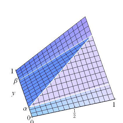
We can develop rich parametric families from the trivial solution with copula $F(x,y) = \min(x,y)$, the case of perfect (positive) correlation, and its counterpart for perfect negative correlation. Concentrating the probability instead along the line segment connecting $(0,\alpha)$ to $(1,\beta)$ with $\beta\gt \alpha$ gives the copula
$$F(x,y;\alpha,\beta) = \cases{\matrix{x y,&0\le y \lt \alpha\text{ or }\beta \lt y \le 1 \\
\beta x,&x(\beta-\alpha)\le y-\alpha \\
\alpha x + y-\alpha&\text{otherwise.}}}$$
A similar copula arises when $\beta \lt \alpha$, which I will also designate $F(x,y;\alpha,\beta)$.

Think of these as mixtures: when $\beta \gt \alpha$, there are uniform components on the horizontal rectangles $[0,1]\times [0,\alpha]$, $[0,1]\times[\beta,1]$, and on the central rectangle $[0,1]\times[\alpha,\beta]$ there is a perfect correlation (whose distribution is that of $(U, \alpha+(\beta-\alpha)U)$ for a uniformly distributed variable $U$). This conception of $F$ makes it easy to compute the regression: it's a weighted sum of the three conditional means,
$$\mathbb{E}(Y\mid X) = \alpha\left(\frac{\alpha}{2}\right) + (\beta-\alpha)\left(\alpha + (\beta-\alpha)X\right) + (1-\beta)\left(\frac{1+\beta}{2}\right).$$
This evidently is linear in $X$: the intercept equals $(1+(\beta-\alpha)^2)/2$ and the slope is $(\beta-\alpha)^2$ times the sign of $\beta-\alpha$. Moreover, it has been constructed to have uniform marginals.
To create a parametric family, choose any parametric distribution for $(\alpha,\beta)$ with parameter $\theta$. Let $G(\alpha,\beta;\theta)$ be the distribution function. It describes a mixture of the $F(;\alpha,\beta)$ via integration:
$$\tilde F(x,y;\theta) = \iint F(x,y;\alpha,\beta)dG(\alpha,\beta;\theta)$$
is the distribution function (copula). Because each $F(;\alpha,\beta)$ has uniform marginals, so does $\tilde F(;\theta)$. Moreover, its regression is linear because
$$\eqalign{
\mathbb{E}_{\tilde F(;\theta)}(Y\mid X) &= \iint \mathbb{E}_{F(;\alpha,\beta)}(Y\mid X)dG(\alpha,\beta;\theta)\\
&=\iint ((1+(\beta-\alpha)^2)/2 + \operatorname{sgn}(\beta-\alpha)(\beta-\alpha)^2 X)dG(\alpha,\beta;\theta) \\
&= \iint (1+(\beta-\alpha)^2)/2 dG(\alpha,\beta;\theta) + \iint \operatorname{sgn}(\beta-\alpha)(\beta-\alpha)^2 dG(\alpha,\beta;\theta)\,X\\
&= \mathbb{E}_{G(;\theta)}((1+(\beta-\alpha)^2)/2) + \mathbb{E}_{G(;\theta)}(\operatorname{sgn}(\beta-\alpha)(\beta-\alpha)^2)X.
}$$
This shows how the intercept and slope are the expectations of the intercept and slope (with respect to $G$), providing useful information for selecting appropriate families $G(;\theta)$.

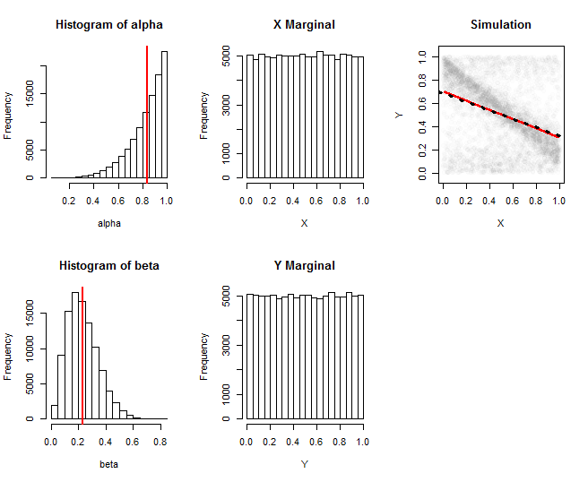
These graphics document a simulation from one such family. Here, $\alpha$ was drawn from a Beta$(5,1)$ distribution and $\beta$ was drawn independently from a Beta$(3,10)$ distribution. The first column shows histograms of the realizations of these parameters. The second column shows histograms of the marginal distributions of $X$ and $Y$: they are satisfactorily close to uniform. The rightmost column shows a random subset of the 100,000 simulated values, along with an estimate of its regression (the red line) and an approximation to the theoretical regression (black dotted line): they agree closely. The estimated regression was obtained by computing the means of $X$ and $Y$ within windows of $X$, then smoothing their trace with Loess.
(The "theoretical" regression line is only an approximation obtained by replacing $\alpha$ and $\beta$ in the expectation formulas by their expectations. Exact formulas are straightforward to work out in this case, but are long and messy to code.)
The R code that produced this figure can readily be used to study other families $G(;\theta)$.
#
# Draw `n` variates from the mixture copula.
# `alpha` and `beta` are intended to be realizations of G(;theta).
#
runif.xy <- function(n, alpha=0, beta=1) {
  a <- pmin(alpha, beta)
  b <- pmax(alpha, beta)
  xy <- matrix(runif(2*n), nrow=2)              # Start with a uniform distribution
  i <- xy[2,] > a & xy[2,] < b                  # Select the middle rectangle
  xy[2, i] <- (xy[1,]*(beta - alpha) + alpha)[i]# Create perfect correlation
  return(xy)
}
#
# Specify the parameters ("theta").
#
a.alpha <- 5
b.alpha <- 1
a.beta <- 3
b.beta <- 10
#
# Draw the slope `beta` and intercept `alpha` from G(;theta).
#
n.sim <- 1e5
alpha <- rbeta(n.sim, a.alpha, b.alpha)
beta <- rbeta(n.sim, a.beta, b.beta)
#
# Draw (X,Y) from the mixture.
#
sim <- runif.xy(n.sim, alpha, beta)
#
# Plot histograms of alpha, beta, X, Y.
#
par(mfcol=c(2,3))
hist(alpha); abline(v=a.alpha/(a.alpha+b.alpha), col="Red", lwd=2)
hist(beta); abline(v=a.beta/(a.beta+b.beta), col="Red", lwd=2)
hist(sim[1,], main="X Marginal", xlab="X")
hist(sim[2,], main="Y Marginal", xlab="Y")
#
# Plot the simulation and its regression curve.
#
i <- sample.int(n.sim, min(5e3, n.sim)) # Limit how many points are shown
plot(t(sim[, i]), asp=1, pch=19, col="#00000002", main="Simulation",
     xlab="X", ylab="Y")

library(zoo)
i <- order(sim[1,])
x <- as.vector(rollapply(ts(sim[1, i]), ceiling(n.sim/100), mean))
y <- as.vector(rollapply(ts(sim[2, i]), ceiling(n.sim/100), mean))
lines(lowess(y ~ x), col="Red", lwd=2)
#
# Overplot the theoretical regression curve.
#
a <- a.alpha / (a.alpha + b.alpha) # Expectation of `alpha`
b <- a.beta / (a.beta + b.beta)    # Expectation of `beta`
intercept <- (1 + (b-a)^2)/2
slope <- (b - a)^2 * sign(b-a)
abline(c(intercept, slope), lty=3, lwd=3)


