3
$\begingroup$

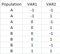
I have an "partially" full factorial designed experiment (3 factors) that looks like this (both VAR1 and VAR2 are numeric factors):

enter image description here

As you can see, Population A and B share all of VAR2 levels and the "0" middle level of VAR1. Is there a name for this type of design?

The model would be

Model: Y = B0+ B1*VAR1 + B2*VAR2 + B3*POP + B4*POPxVAR1 + B5*POPxVAR2

Where Y is the logit and VAR 1 is numeric and VAR 2 is numeric (POP is binary)

I want to estimate the effect of each main effect (VAR 1 and Var 2) for population A and B (i.e. through an interaction) without extrapolating outside of the limits of what factors Population A and B were exposed to.

Questions:

  1. Is this possible (I dont want to just subset the data for separate regressions)?

    2. Will the coefficients be biased from this model?

EDIT #1:

I was actually quite surprised by what happens when you fit a full model to the above data, versus a subset. I think this suggests my concern for bias in the coefficients is not a true concern?

I created some fake data for this, but the large sample sizes are roughly close.

NOTE: Regardless of my coding above, the actual levels are not equally spaced!

Here is the full model:

population<-c(0,0,0,0,1,1,1,1)
VAR1<-c(300,300,500,500,500,500,1000,1000)
VAR2<-c(500,2500,500,2500,500,2500,500,2500)
non_resp<-c(49917,49975,49833,49900,24962,24977,24978,24968)
response<-c(83,25,167,100,38,23,22,32)

Y<-cbind(response,non_resp)
X<-data.frame(population=population,Var1=VAR1,Var2=VAR2)

summary(glm(Y~population+Var1+Var2+population*Var1+population*Var2, data=X, family = binomial))

Which results in these coeff:

Coefficients:
                  Estimate Std. Error z value Pr(>|z|)    
(Intercept)     -7.728e+00  2.655e-01 -29.111  < 2e-16 ***
population       1.207e+00  4.161e-01   2.900  0.00373 ** 
Var1             4.534e-03  5.707e-04   7.946 1.93e-15 ***
Var2            -3.473e-04  5.483e-05  -6.335 2.38e-10 ***
population:Var1 -4.778e-03  6.823e-04  -7.004 2.49e-12 ***
population:Var2  3.038e-04  1.083e-04   2.805  0.00503 ** 

If we subset to only Population =0 the coefficients for Var1 and Var2 are the same, as are the SE

X_sub<-subset(X,population ==0)
Y_sub<-Y[1:4,]
summary(glm(Y_sub~Var1+Var2, data=X_sub, family = binomial))

We get the following:

Coefficients:
              Estimate Std. Error z value Pr(>|z|)    
(Intercept) -7.728e+00  2.655e-01 -29.111  < 2e-16 ***
Var1         4.534e-03  5.707e-04   7.946 1.93e-15 ***
Var2        -3.473e-04  5.483e-05  -6.335 2.38e-10 ***
$\endgroup$
4
  • 1
    $\begingroup$ If this has a name, it would be a $L_8(2^2\times 3)$ mixed-level Taguchi design. So far, I have not been able to find a reference to such a design, and orthogonality of designed experiments was never my forte. $\endgroup$
    – Tavrock
    Commented Feb 13, 2017 at 23:15
  • $\begingroup$ Any thoughts on the analysis from such a design? Biased coefficients? $\endgroup$
    – B_Miner
    Commented Feb 13, 2017 at 23:31
  • $\begingroup$ I added a few items. I was surprised to see what I think suggests no bias. $\endgroup$
    – B_Miner
    Commented Feb 14, 2017 at 1:34
  • 2
    $\begingroup$ The proper name for this is a fractional factorial design. $\endgroup$ Commented Feb 14, 2017 at 4:24

1 Answer 1

1
+150
$\begingroup$

tl;dr: Logistic regression is always biased in the sense that $E[\hat \beta]$ does not exactly equal the true log odds ratio (relevant CV answer). But, you don't have to worry about aliasing, e.g. one effect completely masking another.

Is LR biased here?

Yes; the estimates are nonlinear functions of the data and shit hits the fan from there. Check out the question I linked to in the tl;dr.

I will continue to pontificate because there is more to your question than that.

A smaller model on a subset yields the same results. Why?

Your coeffs stay the same because of the particular way that glm() sets up your regression. To spoil the punchline, what you're calling a main effect is arguably not a main effect -- it's the population A effect, even in the full model. To see why, print the model matrix.

> my_glm = glm(Y~population+Var1+Var2+population*Var1+population*Var2, 
               data=X, family = binomial)
> model.matrix(my_glm)

 (Intercept) population Var1 Var2 population:Var1 population:Var2
           1          0  300  500               0               0
           1          0  300 2500               0               0
           1          0  500  500               0               0
           1          0  500 2500               0               0
           1          1  500  500             500             500
           1          1  500 2500             500            2500
           1          1 1000  500            1000             500
           1          1 1000 2500            1000            2500

You'll see that the upper right quadrant is all zeroes, while the bottom right and bottom left quadrants are identical. (EDIT: this is more clear if you move the population column two spaces to the right.) This is a perfect linear-algebraic storm for two reasons:

  • fitted values of the first four observations are produced only from the "main effect" coefficients.
  • even if the main effects help or hinder the fitted values of the last four observations, this can be exactly mimicked (or undone) by adjusting the interaction coefficients.

The result is that the "main effects" are free to fit themselves to population A, while the interactions make up the difference between the populations. This annoying sonofabitch is called corner-point parameterization. A simpler version arises when your model says $\hat{Y_1} = \beta_0$ and $\hat{Y_2} = \beta_0 + \beta_1$. In this case, the model matrix is $\begin{bmatrix} 1, 0 \\1, 1\end{bmatrix}$, and $\beta_0$ reflects the first observation only.

I personally would rather use parameters with a "grand mean" $\beta_0 + \beta_1/2$ and an "interaction" equaling $\beta_1/2$ that gets subtracted in one case and added for another, but it's your choice about what inference to make. The predictions will stay the same.

Are there multiple indistinguishable effects?

I'm answering this because I think it's what you mean when you ask about bias. The answer is no. Your covariate matrix has full column rank, so no column is a multiple of the others and no change in one coefficient can be perfectly mimicked by tweaking the others. In other words, your model is identifiable, and there is no aliasing present.

> tol = 10^-5
> sum(svd(MM)$d > tol ) == ncol(MM)
TRUE
$\endgroup$
2
  • $\begingroup$ "A smaller model on a subset yields the same results. Why?" is the main part of my question I think. I am still not sure why the main effect of each variable (i.e. for population A) are unaffected by the other rows. Is this the case with any linear model with an interaction term, that essentially it does a subset regression (for lack of a better term)? $\endgroup$
    – B_Miner
    Commented Feb 24, 2017 at 1:23
  • $\begingroup$ Yes. For any model with enough interactions to fit every combination of factor levels separately, the "main effects" in the default glm parameterization will be fitted to the first level of each factor. Think of a simple scenario: $\begin{bmatrix}1\\10\end{bmatrix} = \begin{bmatrix}1 , 0\\1,1\end{bmatrix}* \begin{bmatrix}1\\9\end{bmatrix}$, so the "main effect" is fitted to the first observation while the interaction makes up the difference to the second. $\endgroup$ Commented Feb 24, 2017 at 17:37

Your Answer

By clicking “Post Your Answer”, you agree to our terms of service and acknowledge you have read our privacy policy.

Not the answer you're looking for? Browse other questions tagged or ask your own question.