solid line from a local average series

Question

I have a time series of data taken from a meteorological station, and I have to extract values from it which are located on a precise point of time; problem is that the station time series I have only gives me average values of measures every half an hour. There is some method to get a smoth line from it, so I can take the singular values I need?

this drawing could explain it better: the black lines are the discrete values I have, the blue line is what I want. actually, it doesn't have to be necessarily smooth, it must be the most realistic it can, so it has to respect the average constraint; in other words, the expected value of taking a random point of the solid (blue) line should be the (black) local average value I have now.

if different options exist, and maybe some books explain them, I'd be happy if you tell me.

Answer 1

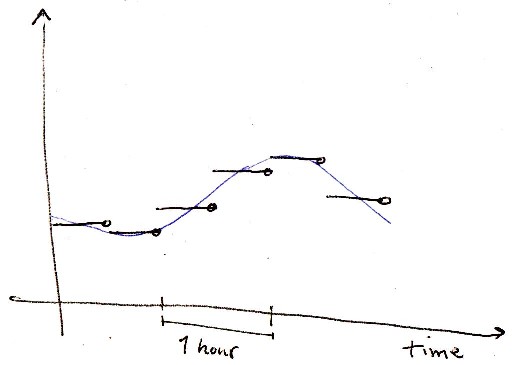
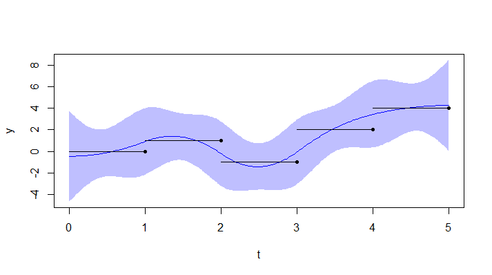
What you want is a mean preserving interpolation. John D'Errico has the exact solution you're looking for, written in MATLAB however.

https://www.mathworks.com/matlabcentral/newsreader/view_thread/31378

function [y,spl]=mean_series(ymeans,n,EndConditions)
% mean_series: cubic spline resampling of series in x
% (n times), maintaining the mean
%
% arguments:
% ymeans - vector of means
% n - 
% EndConditions - flag specifying natural or not-a-knot 
% end conditions on the spline. 
% EndConditions == 0 --> natural
% EndConditions == 1 (default) --> not-a-knot
%
% y - interpolated series, y has the property that:
% ymeans == sum(reshape(y,n,length(x)))
%
% spl - cubic spline as a piecewise cubic Hermite function

% ensure that ymeans is a column vector
ymeans=ymeans(:);
nmeans=length(ymeans);

% things will fail unless there are at least two
% points in ymeans
if nmeans<2
  error 'I require length(ymeans)>=2 or dire things will happen'
end

% nmeans+1 implicit knots
nk=nmeans+1;

% implicit positions of points supplied
xmeans=(0:(nmeans-1))';

% implicit positions of knots
knots=(0:nmeans)'-0.5;

% knot spacing
delta=diff(knots);

% implicit coordinates of the points to be predicted
% (interpolations at these points)
x=linspace(knots(1),knots(end),nmeans*n+1)';
x(end)=[];
ny=n*nmeans;

% define the spline as a piecewise cubic Hermite at
% the knots. This gives us nk function values and
% nk derivatives.

% Force the spline to be C2. compute the matrix
% relating function values to first derivatives,
% comes about from second derivative continuity at
% the knots. these will be equality constraints on
% the unknown spline coefficients.
feq=zeros(nk-2,nk);
deq=zeros(nk-2,nk);
rhseq=zeros(nk-2,1);
for i=2:(nk-1)
  j=i-1;
  feq(j,i+[-1 0 1])=-[-6/delta(j)^2 , ...
      (6/delta(j)^2)-(6/delta(i)^2) , 6/delta(i)^2];
  deq(j,i+[-1 0 1])=[2/delta(j) , ...
      4/delta(j)+4/delta(i) , 2/delta(i)];
end

% next, "evaluate" the points through the implicitly
% defined spline. We do not yet have the coefficients
% defining the spline, but we will eventually.
% k specifies which knot interval the points fall in.
k=repmat(1:nmeans,n,1);
k=k(:);

t=(x-knots(k))./delta(k);
t2=t.*t;
t3=t2.*t;
s2=(1-t).*(1-t);
s3=s2.*(1-t);

% build the matrix sparsely for efficiency, then convert
% the system to full since its really not sparse enough
% to save much.
fmat=[3*s2-2*s3 , 3*t2-2*t3];
dmat=[-delta(k).*(s3-s2) , delta(k).*(t3-t2)];
imat=(1:ny)';
imat=[imat,imat];
jmat=[k,k+1];

fmat0=full(sparse(imat,jmat,fmat,ny,nk));
dmat0=full(sparse(imat,jmat,dmat,ny,nk));

% now, compute implicit means of every n points.
% do it via a matrix multiply.
M=kron(eye(nmeans,nmeans),ones(1,n)/n);
fmat=M*fmat0;
dmat=M*dmat0;

% Since these means are to be forced, specify them
% as equality constraints, appending them to the set
% of equalities.
feq=[feq;fmat];
deq=[deq;dmat];
rhseq=[rhseq;ymeans];

% End condotions are either: 'natural', 'not-a-knot'
% test for default on EndConditions

switch EndConditions
 case 0
  % natural boundary conditions, i.e., zero second
  % derivative at ends
  fe=zeros(2,nk);
  de=zeros(2,nk);
  % at the bottom knot:
  fe(1,1:2)=[-1, 1]*6/(delta(1)^2);
  de(1,1:2)=[-2, -1]*2/delta(1);
  % at the top knot:
  fe(2,nk+[-1 0])=[1, -1]*6/(delta(nk-1)^2);
  de(2,nk+[-1 0])=[1, 2]*2/delta(nk-1);
  % append to equality constraints matrix
  feq=[feq;fe];
  deq=[deq;de];
  rhseq=[rhseq;zeros(2,1)];
case 1
  % not-a-knot end conditions, 3rd derivative continuity at
  % 2nd knot and next to last knots
  fe=zeros(1+(nk>3),nk);
  de=fe;
  % at the second knot:
  fe(1,1:3)=[1 -1 0]*12/(delta(1)^3)-[0 1 -1]*12/(delta(2)^3);
  de(1,1:3)=[1 1 0]*6/(delta(1)^2)-[0 1 1]*6/(delta(2)^2);
  % at the top knot:
  if nk>3
    fe(2,nk+(-2:0))=[1 -1 0]*12/(delta(nk-2)^3)- ...
         [0 1 -1]*12/(delta(nk-1)^3);
    de(2,nk+(-2:0))=[1 1 0]*6/(delta(nk-2)^2)- ...
         [0 1 1]*6/(delta(nk-1)^2);
  end
  % append to equality constraints matrix
  feq=[feq;fe];
  deq=[deq;de];
  rhseq=[rhseq;zeros(1+(nk>3),1)];
end

% the second derivative regularizer is a quadratic form of the form
% s'*regmat*s,
% where s is the vector of (unknown) second derivatives at the knots.
regmat=zeros(nk,nk);
regmat(1,1:2)=[delta(1)/3 , delta(1)/6];
regmat(nk,nk+[-1 0])=[delta(nk-1)/6 , delta(nk-1)/3];

for i=2:(nk-1)
  regmat(i,i+[-1 0 1])=[delta(i-1)/6 , (delta(i-1)+delta(i))/3 , delta(i)/6];
end

% next, write the second derivatives as a function of the
% function values and first derivatives: s = [sf,sd]*[f;d]
sf=zeros(nk,nk);
sd=zeros(nk,nk);
for i=1:(nk-1)
  sf(i,i+[0 1])=[-1 1].*(6/(delta(i)^2));
  sd(i,i+[0 1])=[-4 -2]./delta(i);
end
sf(nk,nk+[-1 0])=[1 -1].*(6/(delta(nk-1)^2));
sd(nk,nk+[-1 0])=[2 4]./delta(nk-1);

regmat=[sf,sd]'*regmat*[sf,sd];

% ensure numerical symmetry of the hessian
regmat=regmat+regmat';

% now, solve this whole mess of a linear system
% using a quadratic programming package.
% assume quadprog from the optimization toolbox 2.0
H=regmat;
f=zeros(2*nk,1);
Aeq=[feq,deq];
beq=rhseq;
options=optimset('quadprog');
coef=quadprog(H,f,[],[],Aeq,beq,[],[],[],options);

% break the coeficients up into a spline.
% first column is the knots, the second column 
% is function values at the knots, the third column
% is first derivatives at the knots.
spl=[knots,reshape(coef,nk,2)];

% return predictions at the original points
y=fmat0*spl(:,2)+dmat0*spl(:,3);

We can test out this function:

ymeans=sin(1:22)';
n=3;
EndConditions=1;

[yhat,spl]=mean_series(ymeans,n,1);

plot(yhat);
hold on
plot(kron(ymeans,ones(n,1)));
hold off

Beautiful!!

Here's yhat, reshaped so that the mean of each row will be equal to the original input:

>> reshape(yhat,3,22)'
ans =

    0.6038    0.8903    1.0303
    1.0413    0.9407    0.7459
    0.4743    0.1473   -0.1983
   -0.5214   -0.7848   -0.9642
   -1.0390   -0.9948   -0.8430
   -0.6010   -0.2903    0.0531
    0.3894    0.6811    0.9005
    1.0219    1.0263    0.9198
    0.7147    0.4279    0.0937
   -0.2493   -0.5639   -0.8188
   -0.9845   -1.0373   -0.9782
   -0.8141   -0.5570   -0.2387
    0.1042    0.4354    0.7210
    0.9276    1.0275    1.0167
    0.8968    0.6749    0.3792
    0.0434   -0.2981   -0.6090
   -0.8525   -0.9972   -1.0344
   -0.9610   -0.7792   -0.5128
   -0.1911    0.1548    0.4860
    0.7618    0.9471    1.0300
    1.0038    0.8673    0.6388
    0.3414   -0.0014   -0.3666

Let's make sure the mean was preserved for each set of n points:

>>yhat_means=kron(eye(length(ymeans)),repmat(1/n,1,n))*yhat;
>>[yhat_means,ymeans]

ans =

    0.8415    0.8415
    0.9093    0.9093
    0.1411    0.1411
   -0.7568   -0.7568
   -0.9589   -0.9589
   -0.2794   -0.2794
    0.6570    0.6570
    0.9894    0.9894
    0.4121    0.4121
   -0.5440   -0.5440
   -1.0000   -1.0000
   -0.5366   -0.5366
    0.4202    0.4202
    0.9906    0.9906
    0.6503    0.6503
   -0.2879   -0.2879
   -0.9614   -0.9614
   -0.7510   -0.7510
    0.1499    0.1499
    0.9129    0.9129
    0.8367    0.8367
   -0.0089   -0.0089

I think this code is extremely satisfying. I've tried to replicate it in R, but I have yet to find a QP solver that works well with equality constraints and no bounds (the Rcplex package might work, but you have to pay for it, which is dumb, since if you're paying for software, you'd pick MATLAB or some other software with decent support). The following R functions/packages that have QP solvers do NOT work for this problem (non-exclusive list): quadprog, ipop, ROI, auglag, nlminb, optimx, trust, COBYLA.

If anyone is interested in that R code, here it is, with one of the dumb solvers (if a good solver becomes available, you can just replace that line, and the code will work as well as the MATLAB implementation - and don't forget to leave a comment here if you find it):

library(alabama)
library(fBasics)

# identity matrix
eye<-function(n){
  if(n==0){
    return(matrix(0,0,0))
  }else{
    M<-matrix(0,n,n)
    M[1+0:(n-1)*(n+1)]<-1
    return(M)
  }
}

# function inspired by matlab's sparse()
sparse<-function(i,j,v,n=0,m=0,nz=0){
  S<-matrix(nz,max(max(i),n),max(max(j),m))
  S[cbind(matrix(i,ncol=1),matrix(j,ncol=1))]<-matrix(v,ncol=1)
  return(S)
}

mean_series<-function(ymeans,n,EndConditions=1,Method="L-BFGS-B"){
  # mean_series: cubic spline resampling of series in x
  # (n times), maintaining the mean
  #
  # arguments:
  # ymeans - vector of means
  # n - 
  # EndConditions - flag specifying natural or not-a-knot 
  # end conditions on the spline. 
  # EndConditions <-<- 0 --> natural
  # EndConditions <-<- 1 (default) --> not-a-knot
  #
  # y - interpolated series, y has the property that:
  # ymeans <-<- sum(reshape(y,n,length(x)))
  #
  # spl - cubic spline as a piecewise cubic Hermite function

  # ensure that ymeans is a column vector
  ymeans<-matrix(ymeans,ncol = 1)
  nmeans<-length(ymeans)

  # things will fail unless there are at least two
  # points in ymeans
  if (nmeans<2){
    stop('I require length(ymeans)><-2 or dire things will happen')
  }

  # nmeans+1 implicit knots
  nk<-nmeans+1

  # implicit positions of knots
  knots<-cbind(0:nmeans)-0.5

  # knot spacing
  delta<-diff(knots)

  # implicit coordinates of the points to be predicted
  # (interpolations at these points)
  x<-seq(knots[1],knots[length(knots)],length.out =nmeans*n+1)
  x<-cbind(x[-length(x)])
  ny<-n*nmeans

  # define the spline as a piecewise cubic Hermite at
  # the knots. This gives us nk function values and
  # nk derivatives.

  # Force the spline to be C2. compute the matrix
  # relating function values to first derivatives,
  # comes about from second derivative continuity at
  # the knots. these will be equality constraints on
  # the unknown spline coefficients.
  feq<-matrix(0,nk-2,nk)
  deq<-matrix(0,nk-2,nk)
  rhseq<-matrix(0,nk-2,1)
  for(i in 2:(nk-1)){
    j<-i-1
    feq[j,i+(-1:1)]<--cbind(-6/delta[j]^2 ,(6/delta[j]^2)-(6/delta[i]^2) , 6/delta[i]^2)
    deq[j,i+(-1:1)]<- cbind(2/delta[j] , 4/delta[j]+4/delta[i] , 2/delta[i])
  }

  # next, "evaluate" the points through the implicitly
  # defined spline. We do not yet have the coefficients
  # defining the spline, but we will eventually.
  # k specifies which knot interval the points fall in.
  k<-matrix(1:nmeans,n*nmeans,1)

  t<-(x-knots[k])/delta[k]
  t2<-t*t
  t3<-t2*t
  s2<-(1-t)*(1-t)
  s3<-s2*(1-t)

  # build the matrix sparsely for efficiency, then convert
  # the system to full since its really not sparse enough
  # to save much.
  fmat<-cbind(3*s2-2*s3 , 3*t2-2*t3)
  dmat<-cbind(-delta[k]*(s3-s2) , delta[k]*(t3-t2))
  imat<-cbind(1:ny)
  imat<-cbind(imat,imat)
  jmat<-cbind(k,k+1)

  fmat0<-sparse(imat,jmat,fmat,ny,nk)
  dmat0<-sparse(imat,jmat,dmat,ny,nk)

  # now, compute implicit means of every n points.
  # do it via a matrix multiply.
  M<-kron(eye(nmeans),matrix(1,1,n)/n)
  fmat<-M%*%fmat0
  dmat<-M%*%dmat0

  # Since these means are to be forced, specify them
  # as equality constraints, appending them to the set
  # of equalities.
  feq<-rbind(feq,fmat)
  deq<-rbind(deq,dmat)
  rhseq<-rbind(rhseq,ymeans)

  # End condotions are either: 'natural', 'not-a-knot'
  # test for default on EndConditions

  if(EndConditions==0){
    # natural boundary conditions, i.e., zero second
    # derivative at ends
    fe<-matrix(0,2,nk)
    de<-matrix(0,2,nk)
    # at the bottom knot:
    fe[1,1:2]<-c(-1, 1)*6/(delta[1]^2)
    de[1,1:2]<-c(-2, -1)*2/delta[1]
    # at the top knot:
    fe[2,nk+(-1:0)]<-c(1,-1)*6/(delta[nk-1]^2)
    de[2,nk+(-1:0)]<-c(1,2)*2/delta[nk-1]
    # append to equality constraints matrix
    feq<-rbind(feq,fe)
    deq<-rbind(deq,de)
    rhseq<-rbind(rhseq,matrix(0,2,1))
  }
  if(EndConditions==1){
    # not-a-knot end conditions, 3rd derivative continuity at
    # 2nd knot and next to last knots
    fe<-matrix(0,1+(nk>3),nk)
    de<-fe
    # at the second knot:
    fe[1,1:3]<-c(1,-1,0)*12/(delta[1]^3)-c(0,1,-1)*12/(delta[2]^3)
    de[1,1:3]<-c(1,1,0)*6/(delta[1]^2)-c(0,1,1)*6/(delta[2]^2)
    # at the top knot:
    if(nk>3){
      fe[2,nk+(-2:0)]<-c(1,-1,0)*12/(delta[nk-2]^3)-c(0,1,-1)*12/(delta[nk-1]^3)
      de[2,nk+(-2:0)]<-c(1,1,0)*6/(delta[nk-2]^2)-c(0,1,1)*6/(delta[nk-1]^2)
    }
    # append to equality constraints matrix
    feq<-rbind(feq,fe)
    deq<-rbind(deq,de)
    rhseq<-rbind(rhseq,matrix(0,1+(nk>3),1))
  }

  # the second derivative regularizer is a quadratic form of the form
  # s'*regmat*s,
  # where s is the vector of (unknown) second derivatives at the knots.
  regmat<-matrix(0,nk,nk)
  regmat[1,1:2]<-cbind(delta[1]/3 , delta[1]/6)
  regmat[nk,nk+(-1:0)]<-cbind(delta[nk-1]/6 , delta[nk-1]/3)

  for(i in 2:(nk-1)){
    regmat[i,i+(-1:1)]<-c(delta[i-1]/6 , (delta[i-1]+delta[i])/3 , delta[i]/6)
  }

  # next, write the second derivatives as a function of the
  # function values and first derivatives: s <- [sf,sd]*[fd]
  sf<-matrix(0,nk,nk)
  sd<-matrix(0,nk,nk)
  for(i in 1:(nk-1)){
    sf[i,i+(0:1)]<-c(-1,1)*(6/(delta[i]^2))
    sd[i,i+(0:1)]<-c(-4,-2)/delta[i]
  }
  sf[nk,nk+(-1:0)]<-c(1,-1)*(6/(delta[nk-1]^2))
  sd[nk,nk+(-1:0)]<-c(2,4)/delta[nk-1]

  regmat<-t(cbind(sf,sd))%*%regmat%*%cbind(sf,sd)

  # ensure numerical symmetry of the hessian
  regmat<-regmat+t(regmat)

  # now, solve this whole mess of a linear system
  # using a quadratic programming package.
  # assume quadprog from the optimization toolbox 2.0
  H<-regmat
  f<-matrix(0,2*nk,1)
  Aeq<-cbind(feq,deq)
  beq<-rhseq


  # THIS QP SOLVER DOESN'T FREAKIN WORK AT ALL.
  coef<-cbind(auglag(cbind(rep(0,dim(H)[1])),
                     fn=function(x){t(x)%*%H%*%x},
                     hin=function(x){Aeq%*%x-beq}, 
                     hin.jac=function(x){Aeq}, 
                     heq=function(x){1}, 
                     heq.jac=function(x){rbind(rep(0,dim(Aeq)[2]))},
                     control.outer = list(method=Method,trace=FALSE,itmax=100))$par)



  # break the coeficients up into a spline.
  # first column is the knots, the second column 
  # is function values at the knots, the third column
  # is first derivatives at the knots.
  spl<-cbind(knots,matrix(coef,nk,2))

  # return predictions at the original points
  y<-fmat0%*%spl[,2]+dmat0%*%spl[,3]
  return(y)
}

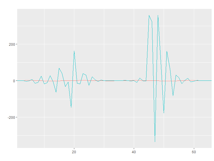
Let's test this stupid QP solver to see how absolutely useless it is:

ymeans<-sin(1:22)
n<-3
yhat<-mean_series(ymeans,n)

lineplot(cbind(kron(ymeans,cbind(rep(1,n))),yhat),1:66,legend = FALSE)

Answer 2

Here's a somewhat more general solution via a computer algebra system (Maxima), which allows for knots at arbitrary places (not fixed intervals) and produces a spline function which can be evaluated at arbitrary places (not fixed intervals). I believe this solution allows the algebraic aspects to be seen more clearly.

Note that QP doesn't come into play. However, the drawback is that, as stated, this isn't easily adapted to a non-symbolic system, although it seems it must be possible to solve the underdetermined system via SVD and then formulate the curvature in terms of the SVD solution.

The full code has been published to Github (constrained_mean_spline.mac) and what's shown here is a lightly abridged version.

Start with the definition of a spline segment.

S[i](u) := a[i] + b[i]*u + c[i]*u^2 + d[i]*u^3;

Approximate data as shown in problem statement above. I've written these numbers as integers and fractions since floating point numbers don't play well with symbolic (exact) solutions.

x: [0, 1/2, 1, 3/2, 2, 5/2, 3];
mu: [1, 9/10, 6/5, 9/5, 2, 7/5];
n: length (mu);

Constraint: mean value on each interval equals a specified value.

eqs_mu: ev (makelist ((integrate (S[i](u), u, x[i], x[i + 1]))/(x[i + 1] - x[i]) = mu[i], i, 1, n), expand);

Constraint: values at endpoints of intervals are equal.

eqs_0: makelist (S[i](x[i + 1]) = S[i + 1](x[i + 1]), i, 1, n - 1);

Constraint: first derivatives at endpoints of intervals are equal.

eqs_1: makelist (at (diff (S[i](u), u, 1), u = x[i + 1]) = at (diff (S[i + 1](u), u, 1), u = x[i + 1]), i, 1, n - 1);

Constraint: second derivatives at endpoints of intervals are equal.

eqs_2: makelist (at (diff (S[i](u), u, 2), u = x[i + 1]) = at (diff (S[i + 1](u), u, 2), u = x[i + 1]), i, 1, n - 1);

At this point we have n + 3*(n - 1) = 4*n - 3 equations. It's conventional to have second derivatives at the end equal to some value, such as zero. That gives two more equations.

eq_d2_0_left: at (diff (S[1](u), u, 2), u = x[1]) = 0;
eq_d2_0_right: at (diff (S[n](u), u, 2), u = x[n + 1]) = 0;

We're still short an equation. Go ahead and solve the equations we have on hand; linsolve will introduce a free parameter that all the coeffcients depend on.

eqs: append (eqs_mu, eqs_0, eqs_1, eqs_2, [eq_d2_0_left, eq_d2_0_right]);

solution: linsolve (eqs, listofvars (eqs));

free_parameter: first (listofvars (map (rhs, solution)));

Final constraint: let's say that the curvature must be minimal, curvature being defined as the integral of the square of the second derivative.

curvature: expand (sum (integrate (diff (S[i](u), u, 2)^2, u, x[i], x[i + 1]), i, 1, n));

curvature_as_function_of_free_parameter: expand (subst (solution, curvature));

eq_curvature_minimum: diff (curvature_as_function_of_free_parameter, free_parameter) = 0;

minimum_curvature_free_parameter: linsolve (eq_curvature_minimum, free_parameter);

minimum_curvature_solution: subst (minimum_curvature_free_parameter, solution);

mininum_curvature_spline_segments: subst (minimum_curvature_solution, makelist (S[i](u), i, 1, n));

At this point we have a list of polynomials that can be used for plotting or evaluation or whatever. The spline segments, plotted separately, can be seen here: spline-segments.svg, and the spline function with each segment restricted to one interval, can be seen here: spline-and-mean-values.svg

Answer 3

I think it's time I closed this Q&A. After a couple of years since asking this question a possible solution came to my mind, which I elaborated into my master thesis. I actually wanted to publish it in some scientific journal, and link the article here, but that turned out to be more difficult than I thought and also not worth the effort since I decided to not pursue a career in academy. Anyhow, my work is not available anywhere, but the end product is here: https://github.com/c-foschi/mapinterval.

Some notes about my solution (from now on Mapinterval) and its relation to other answers:

• Mapinterval corresponds to @ElonPlotkin's answer when the number of computed nodes tend to infinity. In other words, Mapinterval finds the the function that minimizes the integral of the square first derivative, among all functions which first derivative exists on the whole domain.
• I find some similarities between my solution and @RobertDodier's. Mapinterval is also a spline - a quadratic one though, and is also a natural spline since its first derivative is 0 at both ends of the time span.
• Mapinterval uses spline computation methods, and it's fast. Its complexity is O(n).
• I once found a presentation somewhere where they found a solution for this same problem that I think corresponds completely to Mapinterval: they computed the cumulated time series, then they fit a natural cubic spline to that series, and then they computed the derivative of that function.
• One property that was central to my thesis was that Mapinterval is the maximum a-posteriori estimator for the series generating process if we assume that process was Wiener (Brownian Motion). In my thesis I actually wrote that it was the maximum likelihood estimator, but my professor said that my model was properly Bayesian instead. Anyway, this allows us to draw confidence/credibility bands around the estimate, which look really cool:

Answer 4

I think there are a number of methods that suit what you're looking for - some options are: 1. kernel smoothing 2. spline smoothing 3. moving average

There are many more, but I think those three are good candidates. Here is a very nice visual explanation of several smoothing techniques.

The problem is that technically, between $t_a$ and $t_b$, the temperature could take on any value on your measurement scale. Fortunately, since we can probably assume at least moderate time-dependence, the temp at $t_b$ should at be at least partially related to the temp at $t_a$. Choosing a good smoothing method and parameters depends on how strong you think the time dependent effects are, how smooth you want your smoothing function to be, how variable you think think the temp is during the unobserved period.

Hope that helps!