Simulation of Secretary problem: optimal pool size given k=2?

Question

Question:
Is it incorrect to think there is a "sweet spot" where more samples slightly decreases the likelihood of a "Best pick" in the Secretary Problem?

Details:
The "Secretary Problem" from "optimal stopping" is a classic in decision theory. It also relates to the game "deal or no deal", and selection of candidate employees.

It seems here are two "forces" working here: the more samples I have, the more likely that the first ones are far from the max, and the more samples I have the closer the max drawn is to the absolute max.

Here is a single run

1. I uniformly randomly generated N candidates
2. let k = 2 candidates be evaluated but not selected
3. pick the next candidate who is better than the first 2
4. compute the distance between picked candidate and the best drawn candidate and store that.

I wrapped this into a simulation (code below):

• sweep the total candidates from N=5 to N=30
• repeat the process many (n=1e5) times at each N
• (key) I then estimate the quantile where gap is equal to half the domain. This is the place where the results are a wash, where the approach yields a candidate that is half the domain away from the best. (I define this as a "dud".)

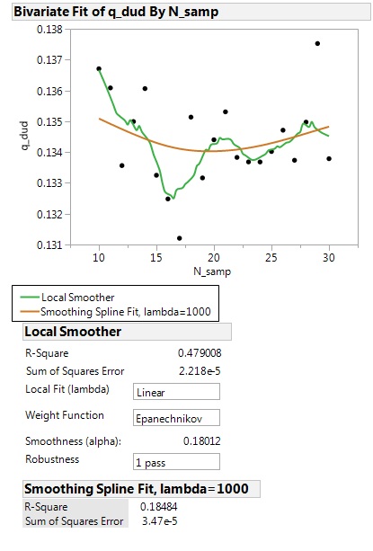
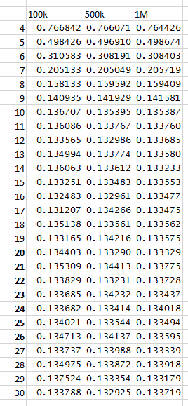
When I run this I get that at N = 10 is a substantial transition in rate of duds, and I am tempted to think it is a plateau. The likelihood of a "dud" here is 13.671%. For all N greater than 10 the percentile is of the form 13.x%. however...

When I:

• plot the quantiles for N >= 10, and use a smoothing spline fit, there is a local minimum at 20
• eyeball the numbers in the table there seems to be an interior minimum
• plot the values, and use a robust kernel fit, there are interior minima.

Is it legitimate to say there is an interior minimum? Is there an analytic, or other, way to dig into this? Did I miss something obvious?

Kernel Fit:

Code:

library(pracma)  #for fzero

N_loops <- 100000 

N_trials <- 25

xz <- numeric()
# set.seed(1)

for (k in 3:30){

     store <- numeric()

     for (i in 1:N_loops){

          y <- runif(n = k)

          best_idx <- which(y==max(y),arr.ind=TRUE)

          do_keep <- FALSE
          my_keep <- 0
          for (j in 1:k){

               #draw one
               yi <- y[j]

               #find in rank
               all_ranks <- rank(y[1:j])
               this_rank <- tail(all_ranks,1)

               #compare with acceptance value
               if (j/exp(1) <1){
                    can_keep = FALSE
               } else {
                    can_keep = TRUE
               }


               #do you keep
               if (can_keep ==TRUE & do_keep == FALSE){
                    if (this_rank >3){
                         do_keep <- TRUE
                         my_keep <- yi
                    }
               }

          }
          store[i] <- my_keep

     }

     store <<- store

     myfit <- function(phi){
          if (phi > 1){
               phi <- 1
          } else if (phi < 0){
               phi <- 0
          }

          err <- quantile(x = store,probs = phi)-0.5
          return(err)
     }

     temp <- fzero(myfit,0.1)
     xz[k] <- unlist(temp)
     print(xz[k]) 
}

Answer 1

I reran this at a million per row, and left it to go all weekend. It look a long time, but the interior minimum went away.

It is a feature of the random number generation and not the physics.