1
$\begingroup$

In a time series, I want to predict $ b_{i+1} $ and I know $ ...,x_{i-1},x_i, x_{i+1} $ and $ ...b_{i-2},b_{i-1},b_i $.

I know by prior knowledge that they have a linear relationship:

$\alpha * x_i = b_i$

Normally I would just make a linear regression to understand the constant $ \alpha $ and find:

$ E[b_{i+1}] = \alpha * x_{i+1}$

But, instead of that what happens if I do this:

$\frac{\alpha * x_{i+1}}{\alpha *x_i } = \frac{b_{i+1}}{b_i}$

Or:

$\frac{x_{i+1}}{x_i} = \frac{b_{i+1}}{b_i}$

$E[b_{i+1}]=b_i*\frac{x_{i+1}}{x_i}$

Instead of estimating the constant $\alpha$, I am in this case estimating the growth rate $\frac{x_{i+1}}{x_i}$. Simulating this millions of time the standard deviation is the same in the two above models.

Example, normal model:

b = > 2,4,8,11,12,15,19,22,31,40

x = > 1,2,4,5 ,6 ,8 ,10,11,15,20

Example, changed model:

b = > 4, 8, 11, 12, 15, 19, 22, 31, 40

x = > 2*2/1, 4*4/2, 8*5/4, 11*6/5, 12*8/6, 15*10/8, 19*11/10, 22*15/11, 31*20/15

My question is: should we predict using past values or is better to ignore $b_i$ despite having it as information? Although $b_i$ is an observed value, not an expected, it is still a real life data. Shouldn't be better for a model to adapt to the real life data?

$\endgroup$
6
  • $\begingroup$ Can't you create a meaningful series/variable using both x and b? $\endgroup$ Commented May 24, 2017 at 20:30
  • $\begingroup$ Also from your third equation, a loglog regression seems to make sense. $\endgroup$ Commented May 24, 2017 at 20:31
  • $\begingroup$ Where is the error term in the linear relationship? $\endgroup$ Commented May 24, 2017 at 20:32
  • $\begingroup$ I'm confused: if $b_i$ is an observed value, then it's by definition real life data. Are both $b_i$ and $x_i$ observed variables (i.e. they are measured separately), or is $x_i$ measured then used to calculate $b_i$ in conjunction with some prior knowledge about $\alpha$? $\endgroup$
    – LmnICE
    Commented May 24, 2017 at 20:39
  • $\begingroup$ @MichaelChernick I am not a Statistician, so correct me if I am wrong. When we make the linear regression to understand the constant $\alpha$ or the growth rate, we will have a intercept and slope. In this case the intercept will "include" the error, thus making it expected value be zero. $\endgroup$
    – Dinidiniz
    Commented May 24, 2017 at 20:53

1 Answer 1

1
$\begingroup$

A regression model must include an error term in order to make sense

\begin{equation} b_i = \alpha \cdot x_i + \epsilon _i \end{equation}

Otherwise, you can't mathematically find a single $\alpha$ that works for all combinations of $(x_i, b_i)$. This is relevant because now it's clearer why your second approach might not work so well: by suggesting that

\begin{equation} E[b_{i+1}] = \alpha \cdot x_{i+1} = \dfrac{b_i}{x_i} \cdot x_{i+1} \end{equation}

you are ignoring the error term $\epsilon _i$:

\begin{align} b_i &= \alpha \cdot x_i + \epsilon _i \\ &\neq \alpha \cdot x_i \end{align}

The average of all error terms must be zero, yes, but any particular $\epsilon _i$ can be arbitrarily large (which would happen if the pair $(x_i, b_i)$ were an outlier)

In other words, the model parameter $\alpha$ contains information about all $N$ $(x_i, b_i)$ pairs. In estimating $E[b_{i+1}]$ using only the information from $(x_i, b_i)$, you are ignoring the information that the pairs $(x_j, b_j) _{j \neq i}$ contain.

As an example, consider your original example:

\begin{align} X_{LV} &= (1, 2, 4, 5, 6, 8, 10, 11, 15, 20, 30) \\ B_{LV} &= (2, 4, 8, 11, 12, 15, 19, 22, 31, 40) \end{align}

Doing the math on the first $N = 10$ elements of both vectors, $\alpha _{LV} = 2.01 \pm 0.08$. You would like to predict the next element in $B_{LV}$, so

\begin{align} E[b_{LV, 11}] &= \alpha _{LV} \cdot x_{LV, 11} \\ &= 60.06 \end{align}

Using your proposed alternative, we get

\begin{align} E'[b_{LV, 11}] &= \dfrac{b_{LV,10}}{x_{LV,10}} \cdot x_{LV, 11} \\ &= 60.0 \end{align}

which represents a $0.1\%$ difference. However, if we run the regression on these series instead

\begin{align} X_{HV} &= (1, 2, 4, 5, 6, 8, 10, 11, 15, 20, 30) \\ B_{HV} &= (2, 4, 8, 11, 12, 15, 19, 22, 21, 47) \end{align}

then we would get an $\alpha _{HV} = 2.0 \pm 0.4$. Note that the slope has a lot more variance in the high variance case. To predict $b_{HV, 11}$ we calculate

\begin{align} E[b_{HV, 11}] &= \alpha _{HV} \cdot x_{HV, 11} \\ &= 59.76 \end{align}

Your proposed alternative, however, yields

\begin{align} E'[b_{HV, 11}] &= \dfrac{b_{HV,10}}{x_{HV,10}} \cdot x_{HV, 11} \\ &= 70.5 \end{align}

which represents a much larger $18\%$ difference. This happens because the pair $(x_{HV,10}, b_{HV,10})$ is an outlier: Comparison between low variance and high variance regressions.
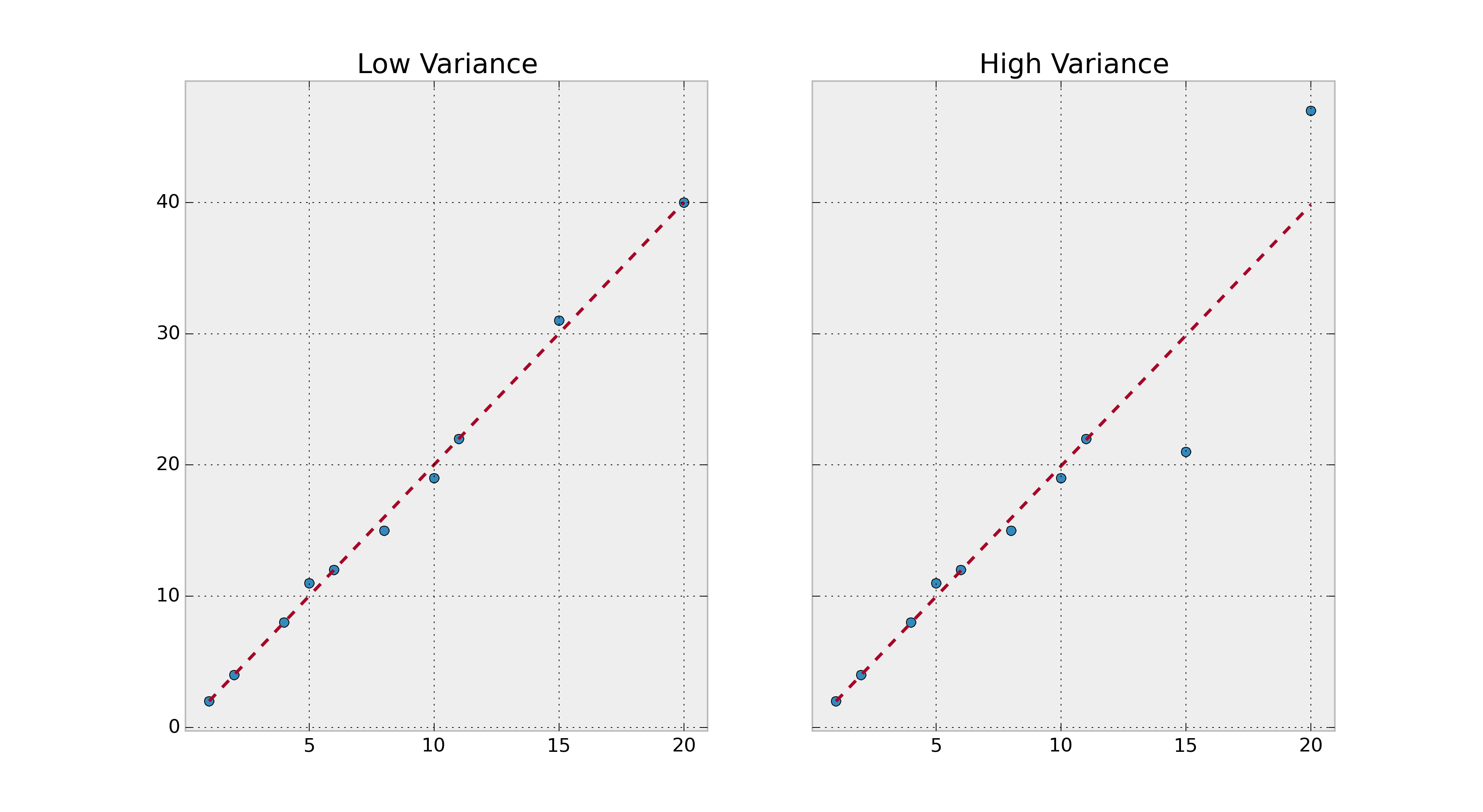
In other words, $\alpha _{HV}$ has information on all $(x_{HV, i}, b_{HV,i}) _{i \in [1\ldots 10]}$ pairs, which results in much better predictions. In contrast, the alternative amplifies any errors present in the $(x_{HV, 10}, b_{HV,10})$ pair.

$\endgroup$
8
  • $\begingroup$ "The average of all error terms must be zero" >> does this follow from the fact that the distribution of the residuals must be normal? $\endgroup$
    – redress
    Commented May 24, 2017 at 21:52
  • $\begingroup$ @redress No. This is what ordinary least squares regression is: find the parameters of a regression model (in this case, the $\alpha$) that minimizes the magnitude of the error terms (the $\epsilon _i$). Mathematically, that is equivalent to setting the mean of the error term distribution to zero, whatever that distribution might be. $\endgroup$
    – LmnICE
    Commented May 24, 2017 at 23:26
  • $\begingroup$ Actually, the two models WORKS in simulations. What I understand of the second model: $E[b_{i+1}] = E[b_i] * E[\frac{x_{i+1}}{x_i}] = E[b_i] * (r + t * \frac{x_{i+1}}{x_i}) $ Where $r$ absorbs the error parameter. So what I see here the difference is that $E[b_i]$ isn't observed $b_i$. But that is for me even better, because your model is adjusting itself to reality. $\endgroup$
    – Dinidiniz
    Commented May 25, 2017 at 4:26
  • $\begingroup$ Two points: 1) When you say the two models work, how are you measuring that? 2) If you're drawing both $x_i$ and $b_i$ from distributions with tight dispersion (low variance), then it makes sense that both approaches seem to work most of the time, because there would be few pairs with a high error term. If either $x_i$ or $b_i$ are drawn from a high variance distribution, then the alternative would not yield good results consistently. If the error term is absorbed by $r$, you wouldn't be able to know whether $r$ is representative of all your data or not unless you ran the regression. $\endgroup$
    – LmnICE
    Commented May 25, 2017 at 11:23
  • $\begingroup$ When I am simulating, the first model is better to predict, showing less variance. When I try to put bigger errors in the simulation, the two models variance grows in the same exponential. But when I use $E[b_i]$ to calculate $b_{i+1}$ instead of $b_i$, the variance of the two models are the same. This is awkward, because I can image situations where the second model is better. For example: in the middle of a time series: $time < X$, all values will be correct; while $time >= X$, all values will be $b_i * 10$; the first model will have problems, the second won't. $\endgroup$
    – Dinidiniz
    Commented May 25, 2017 at 17:05

Your Answer

By clicking “Post Your Answer”, you agree to our terms of service and acknowledge you have read our privacy policy.

Not the answer you're looking for? Browse other questions tagged or ask your own question.