What does it mean for a probability distribution to not have a density function?

Question

I understand the distinction between probability mass and density functions. But I don't understand what it means for a continuous random variable to have a probability distribution but not a density. I am reading this paper where the author consistently refers to the possibility that the probability density $P_{\theta}$ may or may not exist for a probability distribution $\mathbb{P}_{\theta}$. Can anyone explain what it meant by this? I would have thought that if $P_{\theta}$ did not exist, neither would $\mathbb{P}_{\theta}$.

Answer 1

I would suggest to the OP to read Koopmans, L. H. "Teaching singular distributions to undergraduates." The American Statistician 37, no. 4a (1983): 313-316.

My general impression is that "CDF without densities" arise in a way that can be "real-world intuitive" in multivariate settings rather than univariate. As he writes (p. 314)

Finally, whereas singular distributions are difficult (if not impossible) to visualize in one dimension, being distributions concentrated on uncountable zero- dimensional sets (so to speak), in two dimensions they are, or can be constructed to be, concentrated on rather familiar one-dimensional figures such as lines and circles.

He also provides a real-world example indeed (Example 1, p. 314).

Elaborating in a naive way on the bivariate CDF with which he starts, he considers

$$F(x,y) = \frac{x+y}{2},\;\;\;\; 0\leq x\leq 1,\;\; 0\leq y\leq 1.$$

Don't be misled by the notation that "points" towards "continuous distributions". After all this is exactly the issue here.

One can verify that the cross-partial of $F(x,y)$ is zero, $$\frac{\partial^2 F(x,y)}{\partial x \partial y} =0.$$

Strictly speaking the mathematical operation of computing the derivative appears legal, given the information we have, but by giving us the constant zero-function, it leaves us scratching our heads (Koopmans writes "At this point in an exam, it is not unreasonable to expect the normal undergraduate to panic.")

An indication that something peculiar may be going on here is by deriving the marginal CDF, say, for $X$, $$\Pr (X\leq x) = G(x) = \lim_{y\to 1}F(x,y) = \frac{x}{2} + \frac 12.$$ But this means that $\Pr (X=0) = \frac 12$, implying that $X$ is a random variable of "mixed" type (not mixture), and that its marginal CDF $G(x)$ has one continuous and a non-zero discrete component: $$G(x) = \begin{cases} 1/2\qquad\;\;\;\;\;\;\; x=0 \\ 1/2 + x/2 \;\;\;\; 0 < x \leq 1.\end{cases}$$

Koopmans shows that such a mixed distribution leads to a non-zero "singular" component, in the Lebesgue decomposition of a joint density in three parts, one continuous, one discrete and one singular.

Answer 2

As an alternative to Alecos' excellent answer, I will try to give a more intuitive explanation, with the help of two examples.

If the distribution of a random quantity $X$ has a density $\varphi$, numeric values for the probability that $X$ takes values in a given set $A$ can be obtained by integrating $\varphi$ over $A$: $$ P(X\in A) = \int_A \varphi(x) \, dx. $$

If $X$ takes real numbers as values, a consequence of this property is that the probability of $X$ taking any specific value equals zero: $$ P(X = a) = \int_{\{a\}} \varphi(x) \, dx = \int_a^a \varphi(x) \, dx = 0. $$ The following example shows a random quantity which is continuous but has $P(X=0) > 0$ and therefore cannot have a density.

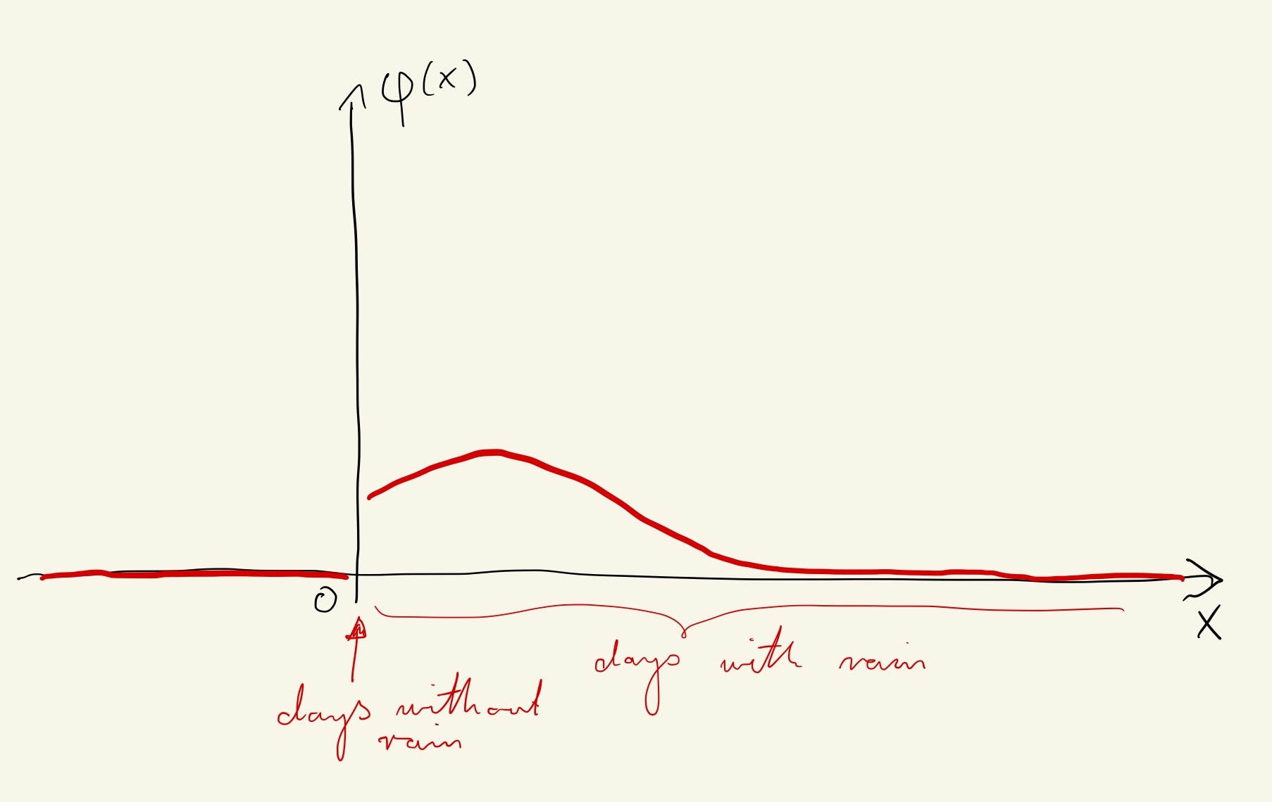
Example 1. Let $X$ be the amount of rainfall in millimetres on this day next year. Clearly the amount of rainfall is a continuous quantity. But where I live there are only 120 days of rain per year, so it seems reasonable to assume $P(X=0) = (365-120)/365 \approx 2/3 > 0$. If we try to find a density for $X$ we may come up with something like the following picture:

The problem is what we should do for $x=0$, where all the days with no rain are represented by a single point on the $x$-axis. To get a density, we would need a "peak" with width 0 and a height such that the integral over the peak equals $P(X=0)$. One might be tempted to set $\phi(0) = \infty$, but even if we accept such a $\phi$ as a valid density, it seems impossible to somehow encode the value $P(X=0) = 2/3$ in the function $\varphi$. Because of these complications, the distribution of $X$ cannot be represented by a density. The distribution can instead be described using a probability measure or the cumulative distribution function.

The same problem also appears in higher dimensions. If $X$ is a random vector with a density, then we still have $P(X=a) = 0$. Similarly, if $A$ is a set with area/volume zero, then the integral discussed above is zero and thus we also must have $P(X\in A) = 0$.

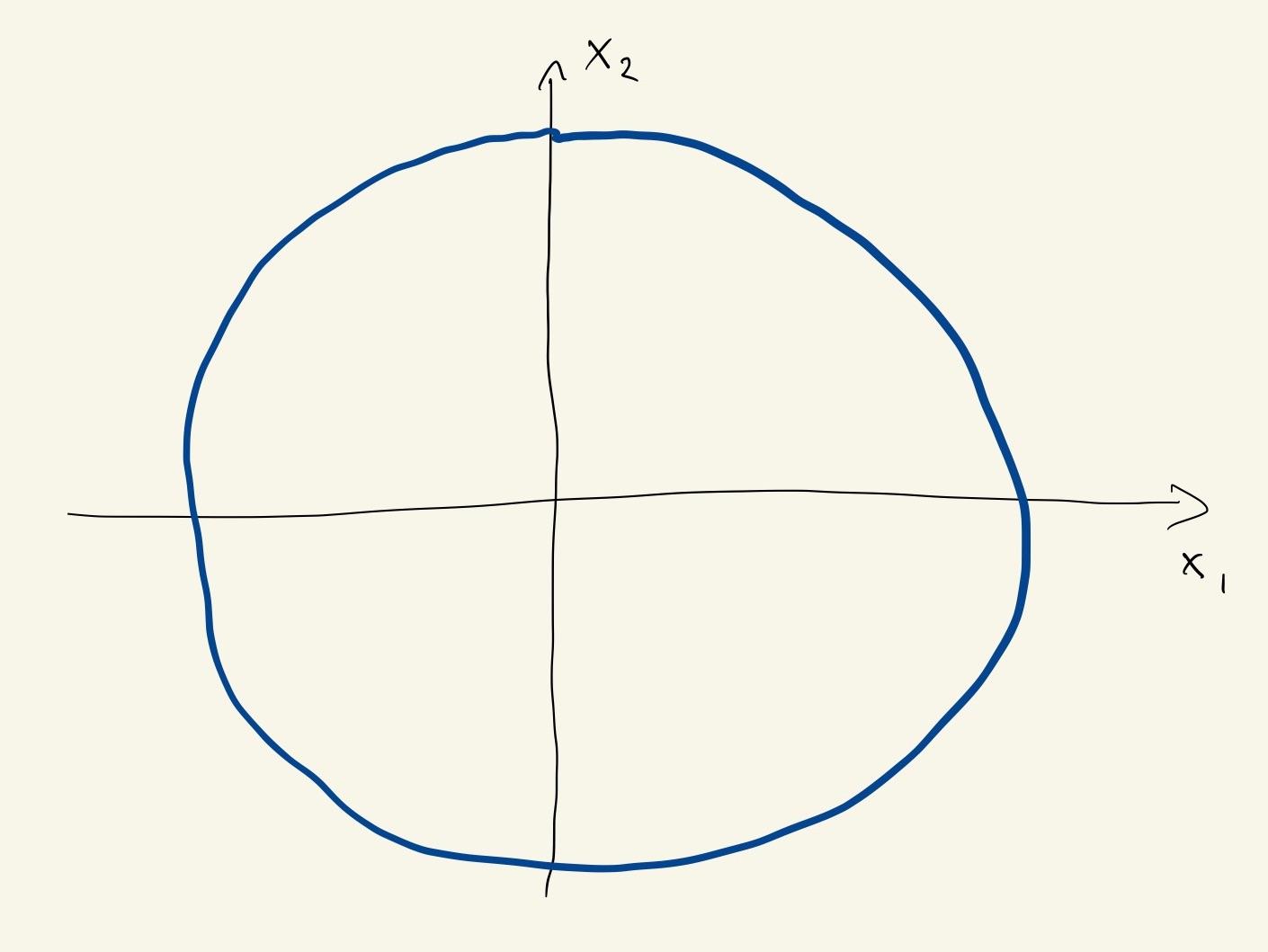
Example 2. Assume that $X = (X_1, X_2)$ is uniformly distributed on the unit circle in the Euclidean plane:

Clearly this is a continuous distribution (there are uncountably many points in the unit circle), but since the circle line has area $0$ it does not contribute to the integral, and any function $\varphi$ with $\varphi(x) = 0$ outside the circle will have $$ \int_{-\infty}^\infty \int_{-\infty}^\infty \varphi(x_1, x_2) \, dx_2 \, dx_1 = 0. $$ Thus there cannot be a density function (integrating to 1) which only takes values on the circle and the distribution of $X$ cannot be described by a density on the Euclidean plane. It can instead be described by a probability measure or by using polar coordinates and using a density just for the angle.