No, the usual formulations of PCA are not convex problems. But they can be transformed into a convex optimization problem.
The insight and the fun of this is following and visualizing the sequence of transformations rather than just getting the answer: it lies in the journey, not the destination. The chief steps in this journey are
Obtain a simple expression for the objective function.
Enlarge its domain, which is not convex, into one which is.
Modify the objective, which is not convex, into one which is, in a way that obviously does not change the points at which it attains its optimal values.
If you keep close watch, you can see the SVD and Lagrange multipliers lurking--but they're just a sideshow, there for scenic interest, and I won't comment on them further.
The standard variance-maximizing formulation of PCA (or at least its key step) is
$$\text{Maximize }f(x)=\ x^\prime \mathbb{A} x\ \text{ subject to }\ x^\prime x=1\tag{*}$$
where the $n\times n$ matrix $\mathbb A$ is a symmetric, positive-semidefinite matrix constructed from the data (usually its sum of squares and products matrix, its covariance matrix, or its correlation matrix).
(Equivalently, we may try to maximize the unconstrained objective $x^\prime \mathbb{A} x / x^\prime x$. Not only is this a nastier expression--it's no longer a quadratic function--but graphing special cases will quickly show it is not a convex function, either. Usually one observes this function is invariant under rescalings $x\to \lambda x$ and then reduces it to the constrained formulation $(*)$.)
Any optimization problem can be abstractly formulated as
Find at least one $x\in\mathcal{X}$ that makes the function $f:\mathcal{X}\to\mathbb{R}$ as large as possible.
Recall that an optimization problem is convex when it enjoys two separate properties:
The domain $\mathcal{X}\subset\mathbb{R}^n$ is convex. This can be formulated in many ways. One is that whenever $x\in\mathcal{X}$ and $y\in\mathcal{X}$ and $0 \le \lambda \le 1$, $\lambda x + (1-\lambda)y\in\mathcal{X}$ also. Geometrically: whenever two endpoints of a line segment lie in $\mathcal X$, the entire segment lies in $\mathcal X$.
The function $f$ is convex. This also can be formulated in many ways. One is that whenever $x\in\mathcal{X}$ and $y\in\mathcal{X}$ and $0 \le \lambda \le 1$, $$f(\lambda x + (1-\lambda)y) \ge \lambda f(x) + (1-\lambda) f(y).$$ (We needed $\mathcal X$ to be convex in order for this condition to make any sense.) Geometrically: whenever $\bar{xy}$ is any line segment in $\mathcal X$, the graph of $f$ (as restricted to this segment) lies above or on the segment connecting $(x,f(x))$ and $(y,f(y))$ in $\mathbb{R}^{n+1}$.
The archetype of a convex function is locally everywhere parabolic with non-positive leading coefficient: on any line segment it can be expressed in the form $y\to a y^2 + b y + c$ with $a \le 0.$
A difficulty with $(*)$ is that $\mathcal X$ is the unit sphere $S^{n-1}\subset\mathbb{R}^n$, which is decidedly not convex. However, we can modify this problem by including smaller vectors. That is because when we scale $x$ by a factor $\lambda$, $f$ is multiplied by $\lambda^2$. When $0 \lt x^\prime x \lt 1$, we can scale $x$ up to unit length by multiplying it by $\lambda=1/\sqrt{x^\prime x} \gt 1$, thereby increasing $f$ but staying within the unit ball $D^n = \{x\in\mathbb{R}^n\mid x^\prime x \le 1\}$. Let us therefore reformulate $(*)$ as
$$\text{Maximize }f(x)=\ x^\prime \mathbb{A} x\ \text{ subject to }\ x^\prime x\le1\tag{**}$$
Its domain is $\mathcal{X}=D^n$ which clearly is convex, so we're halfway there. It remains to consider the convexity of the graph of $f$.
A good way to think about the problem $(**)$--even if you don't intend to carry out the corresponding calculations--is in terms of the Spectral Theorem. It says that by means of an orthogonal transformation $\mathbb P$, you can find at least one basis of $\mathbb{R}^n$ in which $\mathbb A$ is diagonal: that is,
$$\mathbb {A = P^\prime \Sigma P}$$
where all the off-diagonal entries of $\Sigma$ are zero. Such a choice of $\mathbb{P}$ can be conceived of as changing nothing at all about $\mathbb A$, but merely changing how you describe it: when you rotate your point of view, the axes of the level hypersurfaces of the function $x\to x^\prime \mathbb{A} x$ (which were always ellipsoids) align with the coordinate axes.
Since $\mathbb A$ is positive-semidefinite, all the diagonal entries of $\Sigma$ must be non-negative. We may further permute the axes (which is just another orthogonal transformation, and therefore can be absorbed into $\mathbb P$) to assure that $$\sigma_1 \ge \sigma_2 \ge \cdots \ge \sigma_n \ge 0.$$
If we let $x=\mathbb{P}^\prime y$ be the new coordinates $x$ (entailing $y=\mathbb{P}x$), the function $f$ is
$$f(y) = y^\prime \mathbb{A} y = x^\prime \mathbb{P^\prime A P} x = x^\prime \Sigma x = \sigma_1 x_1^2 + \sigma_2 x_2^2 + \cdots + \sigma_n x_n^2.$$
This function is decidedly not convex! Its graph looks like part of a hyperparaboloid: at every point in the interior of $\mathcal X$, the fact that all the $\sigma_i$ are nonnegative makes it curl upward rather than downward.
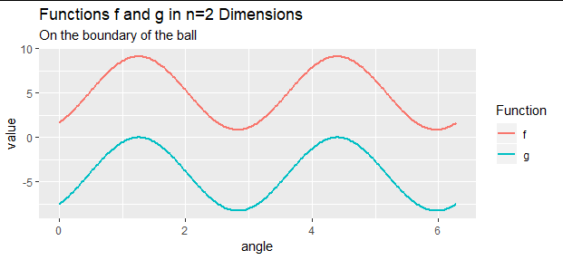
However, we can turn $(**)$ into a convex problem with one very useful technique. Knowing that the maximum will occur where $x^\prime x = 1$, let's subtract the constant $\sigma_1$ from $f$, at least for points on the boundary of $\mathcal{X}$. That will not change the locations of any points on the boundary at which $f$ is optimized, because it lowers all the values of $f$ on the boundary by the same value $\sigma_1$. This suggests examining the function
$$g(y) = f(y) - \sigma_1 y^\prime y.$$
This indeed subtracts the constant $\sigma_1$ from $f$ at boundary points, and subtracts smaller values at interior points. This will assure that $g$, compared to $f$, has no new global maxima on the interior of $\mathcal X$.

Let's examine what has happened with this sleight-of-hand of replacing $-\sigma_1$ by $-\sigma_1 y^\prime y$. Because $\mathbb P$ is orthogonal, $y^\prime y = x^\prime x$. (That's practically the definition of an orthogonal transformation.) Therefore, in terms of the $x$ coordinates, $g$ can be written
$$g(y) = \sigma_1 x_1 ^2 + \cdots + \sigma_n x_n^2 - \sigma_1(x_1^2 + \cdots + x_n^2) = (\sigma_2-\sigma_1)x_2^2 + \cdots + (\sigma_n - \sigma_1)x_n^2.$$
Because $\sigma_1 \ge \sigma_i$ for all $i$, each of the coefficients is zero or negative. Consequently, (a) $g$ is convex and (b) $g$ is optimized when $x_2=x_3=\cdots=x_n=0$. ($x^\prime x=1$ then implies $x_1=\pm 1$ and the optimum is attained when $y = \mathbb{P} (\pm 1,0,\ldots, 0)^\prime$, which is--up to sign--the first column of $\mathbb P$.)

Let's recapitulate the logic. Because $g$ is optimized on the boundary $\partial D^n=S^{n-1}$ where $y^\prime y = 1$, because $f$ differs from $g$ merely by the constant $\sigma_1$ on that boundary, and because the values of $g$ are even closer to the values of $f$ on the interior of $D^n$, the maxima of $f$ must coincide with the maxima of $g$.


