The link ( http://stats.stackexchange.com/questions/141085 ) provided in the comments give great insight. In this post I place some additions and specific comments on the particular biplot function used
I especially recommend you to look at the documentation of the biplot function (in a R console type "?biplot.princomp"). In that documentation you will read that the biplot is based on:
Gabriel, K. R. (1971). The biplot graphical display of matrices with applications to principal component analysis. Biometrika, 58, 453–467.
link
Also the documentation explains you that there are several options to alter the appearance of the plot. For instance your question 1 "Is the upper axis bound to PC1, and the right axis to PC2?" relates to the 'choices' parameter in the function. You can choose different PCs to be on the x and y axis.
As well it is worthwhile to look at the source code of the biplot:
> getS3method("biplot","prcomp")
function (x, choices = 1L:2L, scale = 1, pc.biplot = FALSE, ...)
{
  if (length(choices) != 2L)
    stop("length of choices must be 2")
  if (!length(scores <- x$x))
      stop(gettextf("object '%s' has no scores", deparse(substitute(x))),
          domain = NA)
  if (is.complex(scores))
      stop("biplots are not defined for complex PCA")
  lam <- x$sdev[choices]
  n <- NROW(scores)
  lam <- lam * sqrt(n)
  if (scale < 0 || scale > 1)
      warning("'scale' is outside [0, 1]")
  if (scale != 0)
      lam <- lam^scale
  else lam <- 1
  if (pc.biplot)
      lam <- lam/sqrt(n)
  biplot.default(t(t(scores[, choices])/lam), t(t(x$rotation[,
      choices]) * lam), ...)
  invisible()
}
<bytecode: 0x62870ca8>
<environment: namespace:stats>
with this source code you won't have any confusion about what type of scaling is used (e.g., see that a factor $\sqrt{n}$ is used instead of $\sqrt{n-1}$, the latter being mentioned in an answer to the earlier mentioned question)
Also this scaling stuff answers your question 3. The princomp scales everything by the standard deviation. And the biplot does another scaling with $\sqrt{50}$ as well as the eigenvalues $\lambda$.
The 2d (bi-)plots are essentially projections of multidimensional data. I always believe that a 3d view of PCA is a great help to understand that, and I hope that the following two images may provide you some additional insight for you.
While your data is 4d I took the liberty to eliminate 1 of your
variables in order to make the plotting possible. You will have to
try to extend this idea to some imagination of a higher order
dimensional space.
The biplot:
pok<-matrix(c("Quilava",58,64,58,80,
"Goodra",90,100,70,80,
"Mothim",70,94,50,66,
"Marowak",60,80,110,45,
"Chandelure",60,55,90,80,
"Helioptile",44,38,33,70,
"MeloettaAriaForme",100,77,77,90,
"MetagrossMega",80,145,150,110,
"Sawsbuck",80,100,70,95,
"Probopass",60,55,145,40,
"GiratinaAltered",150,100,120,90,
"Tranquill",62,77,62,65,
"Simisage",75,98,63,101,
"Scizor",70,130,100,65,
"Jigglypuff",115,45,20,20,
"Carracosta",74,108,133,32,
"Ferrothorn",74,94,131,20,
"Kadabra",40,35,30,105,
"Sylveon",95,65,65,60,
"Golem",80,120,130,45,
"Magnemite",25,35,70,45,
"Vanillish",51,65,65,59,
"Unown",48,72,48,48,
"Snivy",45,45,55,63,
"Tynamo",35,55,40,60,
"Duskull",20,40,90,25,
"Beautifly",60,70,50,65,
"Marill",70,20,50,40,
"Lunatone",70,55,65,70,
"Flygon",80,100,80,100,
"Bronzor",57,24,86,23,
"Monferno",64,78,52,81,
"Simisear",75,98,63,101,
"Aromatisse",101,72,72,29,
"Scraggy",50,75,70,48,
"Scolipede",60,100,89,112,
"Staraptor",85,120,70,100,
"GyaradosMega",95,155,109,81,
"Tyrunt",58,89,77,48,
"Zekrom",100,150,120,90,
"Gyarados",95,125,79,81,
"Cobalion",91,90,129,108,
"Espurr",62,48,54,68,
"Spheal",70,40,50,25,
"Dodrio",60,110,70,100,
"Torkoal",70,85,140,20,
"Cacnea",50,85,40,35,
"Trubbish",50,50,62,65,
"Lucario",70,110,70,90,
"GiratinaOrigin",150,120,100,90),50,byrow=1)

pokt <- matrix(as.numeric(pok[,-1]),50)
pokn <- pok[,1]

biplot(pca,scale=1,xlabs=pokn,ylabs=c("attack","defense","speed"),cex=0.7,xlab="",ylab="")
mtext("PCA2 loading of vectors\n multiplied by lambda*sqrt(n)", side=4, line=3)
mtext("PCA1 loading of vectors\n multiplied by lambda*sqrt(n)", side=3, line=2.5)
mtext("PCA2 scores\n divided by lambda*sqrt(n)", side=2, line=2.5)
mtext("PCA1 scores\n divided by lambda*sqrt(n)", side=1, line=3)
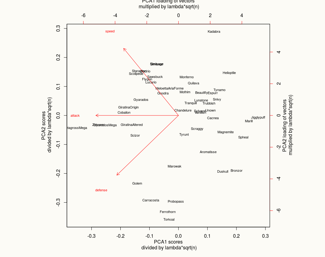
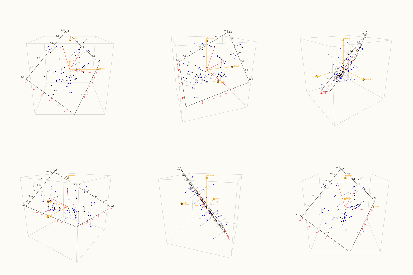
- You should try to see for yourself whether you can recognize the 2d-biplot in the 3d-image.
- Note in the 3d image how the points as well as axes(attack, defense, speed) are projected onto the plane spanned by the PC1 and PC2 vectors.
- points as well as axes (Geometrically a biplot is this two-times projection, showing two things together: the transformed vectors, loadings, as well as the transformed points, scores. Algebraically the biplot is the dual representation of the singular value decomposition matrices $\mathbf{U}$ and $\mathbf{V}$, ands scaled versions thereof.
- in the 3d image the scales do not match the same as the scales in the 2d image. That's because in the 3d image we project both loadings and scores on the same plane, with the same scale in 3d (and we adjust the scales on the edges of the 2d plane), and in the 2d images those scales are placed on different axes allowing to stretch them such that the min and max of the scales coincide$
codeblock for animation (excuse for the dirty writing with little spaces etcetera):
    # centering and scaling
    pokt <- apply(pokt,2, FUN <- function(v) {(v-mean(v))/sqrt(var(v))} )

    # loading libraries (not sure all are needed)
    library("plotrix")
    library(plot3D)
    library(rgl)
    library(matlib)

    # prepare rgl device
    #rgl.close() # for debugging
    rgl.open() # Open a new RGL device
    bgplot3d({
      plot.new()
      title(main = '', line = 3)
    })
    par3d(windowRect = 50 + c( 0, 0, 800, 800 ) )
    rgl.bg(color = "#fcfbf6")
    rgl.viewpoint(theta = -90, phi = 20, zoom = 1)


    # plot data points
    rgl.points(pokt[,2], pokt[,3], pokt[,4], color ="blue",size=5)

    # axes and square box
    N = 2.5

    rgl.lines(c(-N, N), c(-N, -N),c(-N, -N), color = "gray")
    rgl.lines(c(-N, -N), c(-N,N), c(-N, -N), color = "gray")
    rgl.lines(c(-N, -N), c(-N, -N), c(-N,N), color = "gray")
    rgl.lines(c(N, -N), c(N, N), c(N, N), color = "gray")
    rgl.lines(c(N, N), c(N, -N), c(N, N), color = "gray")
    rgl.lines(c(N, N), c(N, N), c(N, -N), color = "gray")
    rgl.lines(c(N, N), c(-N, -N), c(N, -N), color = "gray")
    rgl.lines(c(N, -N), c(N, N), c(-N, -N), color = "gray")
    rgl.lines(c(-N, -N), c(-N, N), c(N, N), color = "gray")
    rgl.lines(c(N, -N), c(-N, -N), c(N, N), color = "gray")
    rgl.lines(c(N, N), c(N, -N), c(-N, -N), color = "gray")
    rgl.lines(c(-N, -N), c(N, N), c(N, -N), color = "gray")

    rgl.lines(c(0, N), c(0, 0),c(0, 0), color = "orange")
    rgl.lines(c(0, 0), c(0, N),c(0, 0), color = "orange")
    rgl.lines(c(0, 0), c(0, 0),c(0, N), color = "orange")
    cone3d(base=c(N,0,0)*0.94,tip=c(N,0,0)*0.06,radius=0.1,col="orange")
    cone3d(base=c(0,N,0)*0.94,tip=c(0,N,0)*0.06,radius=0.1,col="orange")
    cone3d(base=c(0,0,N)*0.94,tip=c(0,0,N)*0.06,radius=0.1,col="orange")

    rgl.texts(c(c(N,0,0),c(0,N,0),c(0,0,N)),
              text = c("attack","defense","speed"), color="orange",
              adj = c(0.0, 0.0), size = 9)

    # biplot calculations
    lam <- pca$sdev[]*sqrt(50)
    scores <-  cbind(pokt[,2],pokt[,3],pokt[,4]) %*% pca$rotation
    scores_sm <- scores %*% diag(lam^-1)

    loadings <- pca$rotation
    loadings_sm <- loadings %*% diag(lam)

    # 2d plot in 3d

       # define boundaries
    max1 <- max(scores[,1])*1.1
    max2 <- max(scores[,2])*1.1
    min1 <- min(scores[,1])*1.1
    min2 <- min(scores[,2])*1.1

       # plot bounding box of biplot
    rgl.lines(c(+max1*pca$rotation[1,1]+max2*pca$rotation[1,2], -max1*pca$rotation[1,1]+max2*pca$rotation[1,2]),
              c(+max1*pca$rotation[2,1]+max2*pca$rotation[2,2], -max1*pca$rotation[2,1]+max2*pca$rotation[2,2]),
              c(+max1*pca$rotation[3,1]+max2*pca$rotation[3,2], -max1*pca$rotation[3,1]+max2*pca$rotation[3,2]),
              color = "black")
    rgl.lines(c(+max1*pca$rotation[1,1]-max2*pca$rotation[1,2], -max1*pca$rotation[1,1]-max2*pca$rotation[1,2]),
              c(+max1*pca$rotation[2,1]-max2*pca$rotation[2,2], -max1*pca$rotation[2,1]-max2*pca$rotation[2,2]),
              c(+max1*pca$rotation[3,1]-max2*pca$rotation[3,2], -max1*pca$rotation[3,1]-max2*pca$rotation[3,2]),
              color = "black")
    rgl.lines(c(+max1*pca$rotation[1,1]+max2*pca$rotation[1,2], +max1*pca$rotation[1,1]-max2*pca$rotation[1,2]),
              c(+max1*pca$rotation[2,1]+max2*pca$rotation[2,2], +max1*pca$rotation[2,1]-max2*pca$rotation[2,2]),
              c(+max1*pca$rotation[3,1]+max2*pca$rotation[3,2], +max1*pca$rotation[3,1]-max2*pca$rotation[3,2]),
              color = "black")
    rgl.lines(c(-max1*pca$rotation[1,1]+max2*pca$rotation[1,2], -max1*pca$rotation[1,1]-max2*pca$rotation[1,2]),
              c(-max1*pca$rotation[2,1]+max2*pca$rotation[2,2], -max1*pca$rotation[2,1]-max2*pca$rotation[2,2]),
              c(-max1*pca$rotation[3,1]+max2*pca$rotation[3,2], -max1*pca$rotation[3,1]-max2*pca$rotation[3,2]),
              color = "black")

    # plot projected points
    projected_points <- scores[,c(1,2)] %*% t(pca$rotation[,c(1,2)])
    rgl.points(projected_points[,1],projected_points[,2],projected_points[,3], color ="black",size=5)

    # plot projection paths for points
    for (i in 1:50) {
      rgl.lines(c(pokt[i,2], projected_points[i,1]),
                c(pokt[i,3], projected_points[i,2]),
                c(pokt[i,4], projected_points[i,3]), color = "gray")
    }

    # plot projected loadings axes
    projected_lines <- N*loadings[,c(1,2)] %*% t(pca$rotation)[c(1,2),]

    rgl.lines(c(0,projected_lines[1,1]),
              c(0,projected_lines[1,2]),
              c(0,projected_lines[1,3]), color="red")

    rgl.lines(c(0,projected_lines[2,1]),
              c(0,projected_lines[2,2]),
              c(0,projected_lines[2,3]), color="red")

    rgl.lines(c(0,projected_lines[3,1]),
              c(0,projected_lines[3,2]),
              c(0,projected_lines[3,3]), color="red")


    # plot tickmarks
    for (i in -3:3) {
      pos = i/10*sqrt(50)*pca$sdev[2]
      rgl.lines(c(-max1*pca$rotation[1,1]+pos*pca$rotation[1,2], -1.05*max1*pca$rotation[1,1]+pos*pca$rotation[1,2]),
                c(-max1*pca$rotation[2,1]+pos*pca$rotation[2,2], -1.05*max1*pca$rotation[2,1]+pos*pca$rotation[2,2]),
                c(-max1*pca$rotation[3,1]+pos*pca$rotation[3,2], -1.05*max1*pca$rotation[3,1]+pos*pca$rotation[3,2]),
                color = "black")
      rgl.texts(-1.08*max1*pca$rotation[1,1]+pos*pca$rotation[1,2],
               -1.08*max1*pca$rotation[2,1]+pos*pca$rotation[2,2],
               -1.08*max1*pca$rotation[3,1]+pos*pca$rotation[3,2],
               text=i/10,color="black")
    }

    for (i in -3:3) {
      pos = i/10*sqrt(50)*pca$sdev[1]
      rgl.lines(c(-max2*pca$rotation[1,2]+pos*pca$rotation[1,1], -1.06*max2*pca$rotation[1,2]+pos*pca$rotation[1,1]),
                c(-max2*pca$rotation[2,2]+pos*pca$rotation[2,1], -1.06*max2*pca$rotation[2,2]+pos*pca$rotation[2,1]),
                c(-max2*pca$rotation[3,2]+pos*pca$rotation[3,1], -1.06*max2*pca$rotation[3,2]+pos*pca$rotation[3,1]),
                color = "black")
      rgl.texts(-1.1*max2*pca$rotation[1,2]+pos*pca$rotation[1,1],
                -1.1*max2*pca$rotation[2,2]+pos*pca$rotation[2,1],
                -1.1*max2*pca$rotation[3,2]+pos*pca$rotation[3,1],
                text=i/10,color="black")
    }

    for (i in -3:2) {
      pos = N*i*2/sqrt(50)/pca$sdev[1]
      rgl.lines(c(max2*pca$rotation[1,2]+pos*pca$rotation[1,1], 1.05*max2*pca$rotation[1,2]+pos*pca$rotation[1,1]),
                c(max2*pca$rotation[2,2]+pos*pca$rotation[2,1], 1.05*max2*pca$rotation[2,2]+pos*pca$rotation[2,1]),
                c(max2*pca$rotation[3,2]+pos*pca$rotation[3,1], 1.05*max2*pca$rotation[3,2]+pos*pca$rotation[3,1]),
                color = "red")
      rgl.texts(1.08*max2*pca$rotation[1,2]+pos*pca$rotation[1,1],
                1.08*max2*pca$rotation[2,2]+pos*pca$rotation[2,1],
                1.08*max2*pca$rotation[3,2]+pos*pca$rotation[3,1],
                text=i*2,color="red")
    }

    for (i in -3:2) {
      pos = N*i*2/sqrt(50)/pca$sdev[2]
      rgl.lines(c(max1*pca$rotation[1,1]+pos*pca$rotation[1,2], 1.05*max1*pca$rotation[1,1]+pos*pca$rotation[1,2]),
                c(max1*pca$rotation[2,1]+pos*pca$rotation[2,2], 1.05*max1*pca$rotation[2,1]+pos*pca$rotation[2,2]),
                c(max1*pca$rotation[3,1]+pos*pca$rotation[3,2], 1.05*max1*pca$rotation[3,1]+pos*pca$rotation[3,2]),
                color = "red")
      rgl.texts(1.08*max1*pca$rotation[1,1]+pos*pca$rotation[1,2],
                1.08*max1*pca$rotation[2,1]+pos*pca$rotation[2,2],
                1.08*max1*pca$rotation[3,1]+pos*pca$rotation[3,2],
                text=i*2,color="red")
    }

    # make movei and close device
    movie3d(spin3d(axis = c(0, 1, 0),rpm=-7.5), duration = 8, fps=10, dir = "~/gif")
    rgl.close()

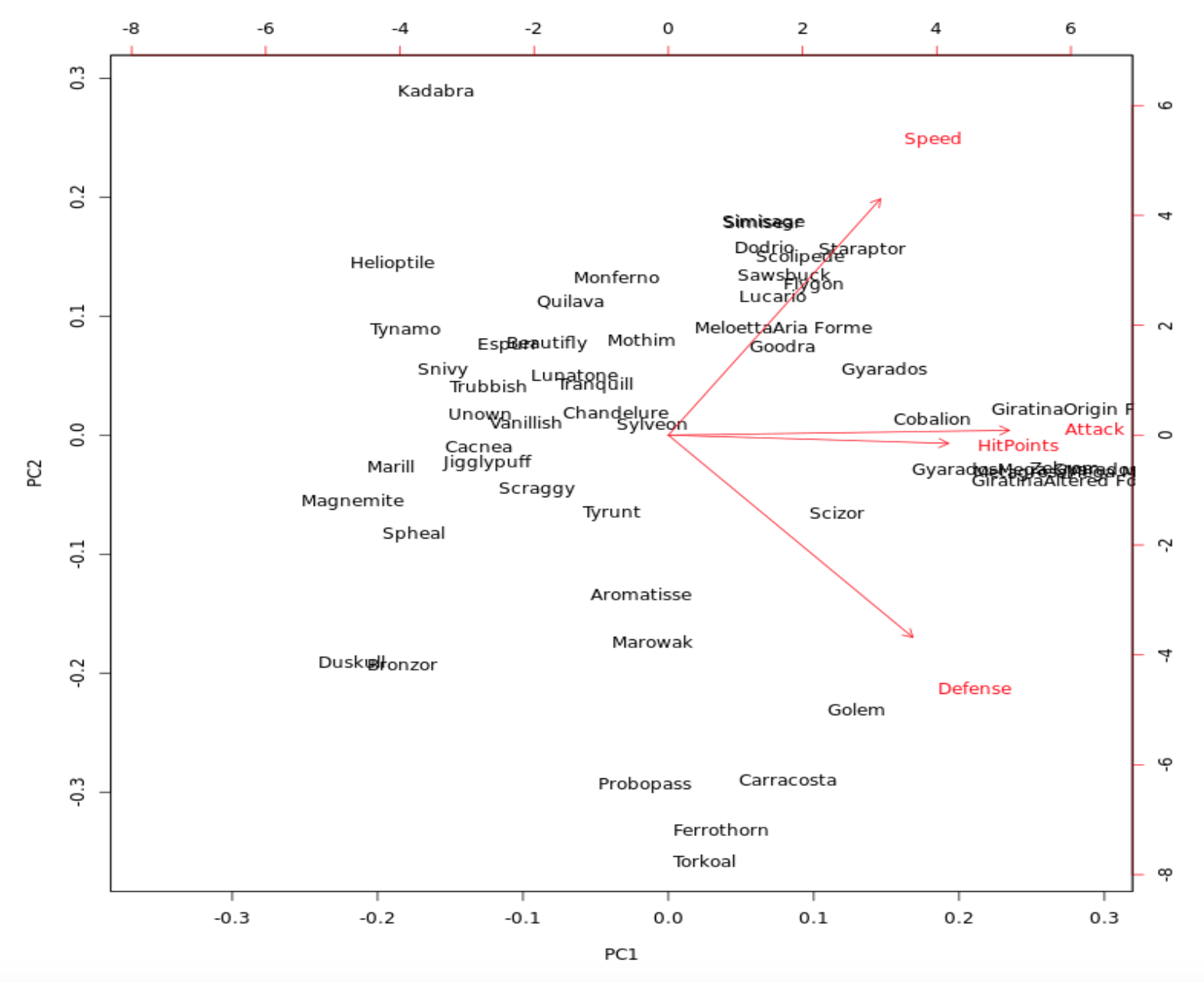


The left and bottom axis are correlations- this is wrong. As written in the linked thread, bottom/left axes show normalized (to unit sum of squares) PC1 and PC2 scores. Regarding your questions, (1) Yes, (2) Yes, (3) These values correspond to PCA eigenvectors (that you see in theprcompoutput) scaled by the PCA eigenvalues and scaled further by the $\sqrt{n}$. All of that is extensively covered on our website and some relevant threads are linked in the thread you read, e.g. see stats.stackexchange.com/questions/141085. $\endgroup$