2
$\begingroup$

I have a data as follows

Date    Paid
Jan-14  13392905
Feb-14  11939873
Mar-14  12473667
Apr-14  12237110
May-14  12579693
Jun-14  12030095
Jul-14  12052101
Aug-14  10205025
Sep-14  12102526
Oct-14  1237336
Nov-14  12148331
Dec-14  9842860
Jan-15  11990085
Feb-15  11061740
Mar-15  12076397
Apr-15  11702514
May-15  11395657
Jun-15  11817594
Jul-15  11643682
Aug-15  10243241
Sep-15  12233001
Oct-15  11769231
Nov-15  12652418
Dec-15  9774333
Jan-16  11888965
Feb-16  11892589
Mar-16  11419517
Apr-16  12143787
May-16  12330387
Jun-16  11929805
Jul-16  11583281
Aug-16  11995557
Sep-16  12646047
Oct-16  12677372
Nov-16  13301244
Dec-16  9915846

Using 2014-2015 information I want to generate forecasts until 2020.Hence, I have split the data into train & test

  data.train<-window(mydata_ts,start=c(2014,1),end=c(2015,12))
  data.test<-window(mydata_ts,start=c(2016,1))
  auto.arima(data.train,trace=TRUE,test="kpss",ic="aic")

& following are the results:

  Best model: ARIMA(0,0,0)            with non-zero mean 

  Series: data.train 
  ARIMA(0,0,0) with non-zero mean 

  Coefficients:
        mean
  11275058.9
  s.e.    463612.8

  sigma^2 estimated as 5.381e+12:  log likelihood=-385.31
  AIC=774.62   AICc=775.19   BIC=776.98

& I get flat forecasts.I have tried using drift but that only helps when forecasting for 2016 & flattens 2017 onward. Is there something that can be done to overcome this.I have also tried the similar exercise in SAS using proc UCM & that seems to generate forecasts better than the auto.arima.

Can someone help out?

$\endgroup$

3 Answers 3

1
$\begingroup$
library(forecast)
library(tsoutliers)

data.train<-window(mydata_ts,start=c(2014,1),end=c(2015,12))
data.test<-window(mydata_ts,start=c(2016,1))

tso_res <- tso(data.train)
tso_res

Series: data.train 
Regression with ARIMA(1,1,0) errors 

Coefficients:
          ar1         AO8         AO10      AO12        AO20        AO24
      -0.8863  -1602271.0  -10339290.5  -1487097  -1552253.1  -2095283.0
s.e.   0.1156    332809.5     384994.5    334836    272327.7    379263.1

sigma^2 estimated as 1.805e+11:  log likelihood=-327.99
AIC=669.99   AICc=677.45   BIC=677.94

Outliers:
  type ind    time   coefhat   tstat
1   AO   8 2014:08  -1602271  -4.814
2   AO  10 2014:10 -10339291 -26.856
3   AO  12 2014:12  -1487097  -4.441
4   AO  20 2015:08  -1552253  -5.700
5   AO  24 2015:12  -2095283  -5.525

plot(tso_res)

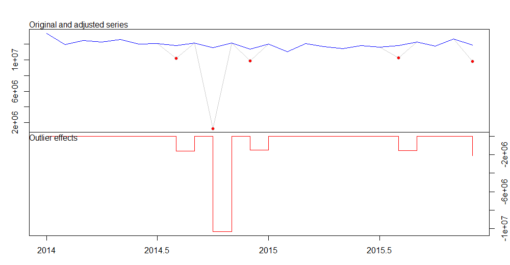
enter image description here

This is the outliers adjusted time series.

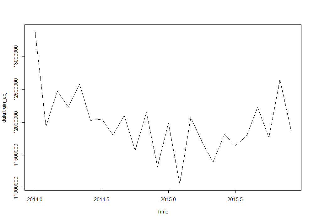
data.train_adj <- tso_res$yadj
plot(data.train_adj)

enter image description here

We can see both data.train and data.train_adj.

> data.train
          Jan      Feb      Mar      Apr      May      Jun      Jul      Aug      Sep      Oct      Nov      Dec
2014 13392905 11939873 12473667 12237110 12579693 12030095 12052101 10205025 12102526  1237336 12148331  9842860
2015 11990085 11061740 12076397 11702514 11395657 11817594 11643682 10243241 12233001 11769231 12652418  9774333
> data.train_adj
          Jan      Feb      Mar      Apr      May      Jun      Jul      Aug      Sep      Oct      Nov      Dec
2014 13392905 11939873 12473667 12237110 12579693 12030095 12052101 11807296 12102526 11576627 12148331 11329957
2015 11990085 11061740 12076397 11702514 11395657 11817594 11643682 11795494 12233001 11769231 12652418 11869616

To accomplish with your need to capture seasonality, I take advantage of dynamic harmonic regression within ARIMA modeling. You may determine an optimal number of Fourier sin and cos pairs number (K) by trying out a pool of values for and select the one with minimum AICc. Here I show it with K=4. Please note that Fourier coefficients are actually not statistically significative as their standard deviations compaired to the coefficients value show.

model_auto <- auto.arima(data.train_adj, trace=TRUE,  ic="aic", stepwise = FALSE, xreg= fourier(data.train_adj, K = 4))
model_auto

Series: data.train_adj 
Regression with ARIMA(1,1,0) errors 

Coefficients:
          ar1      S1-12     C1-12      S2-12     C2-12     S3-12     C3-12    S4-12     C4-12
      -0.8934  -59902.58  101672.4  -81457.95  35595.59  20279.40  67730.84  47447.4  22978.35
s.e.   0.1028  112888.52  102427.8   63037.36  60833.99  53262.02  53310.64  61555.9  60441.30

sigma^2 estimated as 1.799e+11:  log likelihood=-325.75
AIC=671.51   AICc=689.84   BIC=682.86


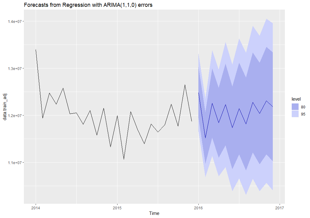
autoplot(forecast(model_auto, xreg=fourier(data.train_adj, K=4, h=12)))

enter image description here

$\endgroup$
3
  • $\begingroup$ Your sine/cosine features are more correctly and more clearly reflected/characterized in Tom's answer . Concluding that there just two months of the year are important is "information extraction" as a result of Exploratory Data Analysis. (EDA) . The anomaly at period 10 ... needs to be identified and it's effect isolated not ignored as is so with your approach which believes the data rather than challenging the data for homogeneity.. I believe you are fitting not modelling in the larger sense. $\endgroup$
    – IrishStat
    Commented Nov 30, 2018 at 17:15
  • $\begingroup$ Actually I adjusted for the outliers when determining the data.train_adj time series. Anyway I agree with you as the dynamic harmonic regression coefficients are not statistically significative. $\endgroup$
    – GiorgioG
    Commented Nov 30, 2018 at 19:56
  • $\begingroup$ urbandictionary.com/define.php?term=gratzi $\endgroup$
    – IrishStat
    Commented Nov 30, 2018 at 20:12
0
$\begingroup$

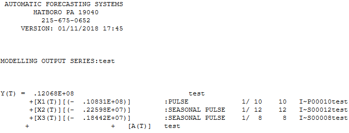
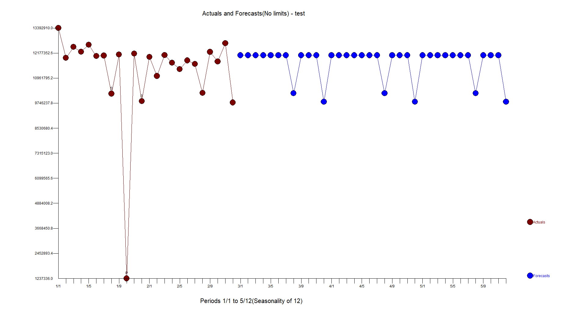
Auto.arima doesn't look for seasonal pulses. It's either all or nothing when it comes to seasonality. Your data has big dips in August and December for both years. Two seasonal dummies (ie seasonal pulse) are identified by Autobox (a software I helped to develop) Model developed.

There is also a very low value at the 10th period which should be identified as an outlier(this is only 24 observations so this a short dataset). UCM doesn't look for outliers nor does auto.arima.

Actual/Forecast

$\endgroup$
4
  • 1
    $\begingroup$ Thanks Tom.Yes I did notice it when I began modeling.However, what can best be done to generate forecasts under such a circumstance. Will plugging in seasonality help? $\endgroup$
    – New2015
    Commented Jan 15, 2018 at 15:57
  • $\begingroup$ Does the low August and December make sense? If so, then yes. $\endgroup$
    – Tom Reilly
    Commented Jan 16, 2018 at 14:38
  • $\begingroup$ Yes it does.But can you guide me as to how do I plug in seasonality variables. I cannot use autobox as it is not available for download in my organization. I tried running proc ucm in SAS & included the season variable. How can the same be done efficiently in r ? $\endgroup$
    – New2015
    Commented Jan 16, 2018 at 16:40
  • $\begingroup$ I have no reason to use R. $\endgroup$
    – Tom Reilly
    Commented Jan 26, 2018 at 16:41
0
$\begingroup$

There is barely any trend in your data. How do you expect to get anything but a flat forecast? Simple regression (err, graphing and trendline in Excel) of this data (ignoring the huge dip in Oct-14) give you a monthly trend of +$3876 per week, which is approximately +.02% per month. Do you not have access to weekly data? more data would be better, especially if you want to train this ARIMA model.

$\endgroup$

Your Answer

By clicking “Post Your Answer”, you agree to our terms of service and acknowledge you have read our privacy policy.

Not the answer you're looking for? Browse other questions tagged or ask your own question.