14
$\begingroup$

Batch normalization has been credited with substantial performance improvements in deep neural nets. Plenty of material on the internet shows how to implement it on an activation-by-activation basis. I've already implemented backprop using matrix algebra, and given that I'm working in high-level languages (while relying on Rcpp (and eventually GPU's) for dense matrix multiplication), ripping everything out and resorting to for-loops would probably slow my code substantially, in addition to being a huge pain.

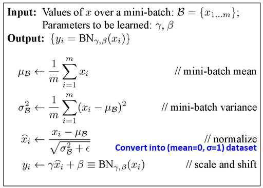
The batch normalization function is $$ b(x_p) = \gamma \left(x_p - \mu_{x_p}\right) \sigma^{-1}_{x_p} + \beta $$ where

  • $x_p$ is the $p$th node, before it gets activated
  • $\gamma$ and $\beta$ are scalar parameters
  • $\mu_{x_p}$ and $\sigma_{x_p}$ are the mean and SD of $x_p$. (Note that the square root of of the variance plus a fudge factor is normally used -- let's assume nonzero elements for compactness)

In matrix form, batch normalization for a whole layer would be $$ b(\mathbf{X}) = \left(\gamma\otimes\mathbf{1}_p\right)\odot \left(\mathbf{X} - \mu_{\mathbf{X}}\right) \odot\sigma^{-1}_{\mathbf{X}} + \left(\beta\otimes\mathbf{1}_p\right) $$ where

  • $\mathbf{X}$ is $N\times p$
  • $\mathbf{1}_N$ is a column vector of ones
  • $\gamma$ and $\beta$ are now row $p$-vectors of the per-layer normalization parameters
  • $\mu_{\mathbf{X}}$ and $\sigma_{\mathbf{X}}$ are $N \times p$ matrices, where each column is a $N$-vector of columnwise means and standard deviations
  • $\otimes$ is the Kronecker product and $\odot$ is the elementwise (Hadamard) product

A very simple one-layer neural net with no batch normalization and a continuous outcome is $$ y = a\left(\mathbf{X\Gamma}_1\right)\Gamma_2 + \epsilon $$

where

  • $\Gamma_1$ is $p_1 \times p_2$
  • $\Gamma_2$ is $p_2 \times 1$
  • $a(.)$ is the activation function

If the loss is $R = N^{-1}\displaystyle\sum\left(y - \hat{y}\right)^2$, then the gradients are $$ \begin{array}{lr} \frac{\partial R}{\partial \Gamma_1} = -2\mathbf{V}^T \hat\epsilon\\ \frac{\partial R}{\partial \Gamma_2} = \mathbf{X}^T \left(a'(\mathbf{X}\mathbf{\Gamma}_1) \odot -2\hat\epsilon \mathbf{\Gamma}_2^T\right) \\ \end{array} $$

where

  • $\mathbf{V} = a\left(\mathbf{X}\Gamma_1\right)$
  • $\hat{\epsilon} = y-\hat{y}$

Under batch normalization, the net becomes $$ y = a\left(b\left(\mathbf{X}\Gamma_1\right)\right)\Gamma_2 $$ or $$ y = a\Big(\left(\gamma\otimes\mathbf{1}_N\right)\odot \left(\mathbf{X\Gamma_1} - \mu_{\mathbf{X\Gamma_1}}\right) \odot\sigma^{-1}_{\mathbf{X\Gamma_1}} + \left(\beta\otimes\mathbf{1}_N\right)\Big)\mathbf{\Gamma_2} $$ I have no idea how to compute the derivatives of Hadamard and Kronecker products. On the subject of Kronecker products, the literature gets fairly arcane.

Is there a practical way of computing $\partial R/\partial \gamma$, $\partial R/\partial \beta$, and $\partial R/\partial \mathbf{\Gamma_1}$ within the matrix framework? A simple expression, without resorting to node-by-node computation?

Update 1:

I've figured out $\partial R/\partial \beta$ -- sort of. It is: $$ \mathbf{1}_{N}^T \left(a'(\mathbf{X}\mathbf{\Gamma}_1) \odot -2\hat\epsilon \mathbf{\Gamma}_2^T\right) $$ Some R code demonstrates that this is equivalent to the looping way to do it. First set up the fake data:

set.seed(1)
library(dplyr)
library(foreach)

#numbers of obs, variables, and hidden layers
N <- 10
p1 <- 7
p2 <- 4
a <- function (v) {
  v[v < 0] <- 0
  v
}
ap <- function (v) {
  v[v < 0] <- 0
  v[v >= 0] <- 1
  v
}

# parameters
G1 <- matrix(rnorm(p1*p2), nrow = p1)
G2 <- rnorm(p2)
gamma <- 1:p2+1
beta <- (1:p2+1)*-1
# error
u <- rnorm(10)

# matrix batch norm function
b <- function(x, bet = beta, gam = gamma){
  xs <- scale(x)
  gk <- t(matrix(gam)) %x% matrix(rep(1, N))
  bk <- t(matrix(bet)) %x% matrix(rep(1, N))
  gk*xs+bk
}
# activation-wise batch norm function
bi <- function(x, i){
  xs <- scale(x)
  gk <- t(matrix(gamma[i]))
  bk <- t(matrix(beta[i]))
  suppressWarnings(gk*xs[,i]+bk)
}

X <- round(runif(N*p1, -5, 5)) %>% matrix(nrow = N)
# the neural net
y <- a(b(X %*% G1)) %*% G2 + u

Then compute derivatives:

# drdbeta -- the matrix way
drdb <- matrix(rep(1, N*1), nrow = 1) %*% (-2*u %*% t(G2) * ap(b(X%*%G1)))
drdb
           [,1]      [,2]    [,3]        [,4]
[1,] -0.4460901 0.3899186 1.26758 -0.09589582
# the looping way
foreach(i = 1:4, .combine = c) %do%{
  sum(-2*u*matrix(ap(bi(X[,i, drop = FALSE]%*%G1[i,], i)))*G2[i])
}
[1] -0.44609015  0.38991862  1.26758024 -0.09589582

They match. But I'm still confused, because I don't really know why this works. The MatCalc notes referenced by @Mark L. Stone say that the derivative of $\beta \otimes \mathbf{1}_N$ should be

$$ \frac{\partial A \otimes B}{\partial A} = \left(I_{nq} \otimes T_{mp}\right)\left(I_n\otimes vec(B) \otimes I_m\right) $$ where the subscripts $m$, $n$, and $p$, $q$ are the dimensions of $A$ and $B$. $T$ is the commutation matrix, which is just 1 here because both inputs are vectors. I try this and get a result that doesn't seem helpful:

# playing with the kroneker derivative rule
A <- t(matrix(beta)) 
B <- matrix(rep(1, N))
diag(rep(1, ncol(A) *ncol(B))) %*% diag(rep(1, ncol(A))) %x% (B) %x% diag(nrow(A))
     [,1] [,2] [,3] [,4]
 [1,]    1    0    0    0
 [2,]    1    0    0    0
 snip
[13,]    0    1    0    0
[14,]    0    1    0    0
snip
[28,]    0    0    1    0
[29,]    0    0    1    0
[snip
[39,]    0    0    0    1
[40,]    0    0    0    1

This isn't conformable. Clearly I'm not understanding those Kronecker derivative rules. Help with those would be great. I'm still totally stuck on the other derivatives, for $\gamma$ and $\mathbf{\Gamma_1}$ -- those are harder because they don't enter additively like $\beta \otimes \mathbf{1}$ does.

Update 2

Reading textbooks, I'm fairly sure that $\partial R/\partial \Gamma_1$ and $\partial R/\partial \gamma$ will require use of the vec() operator. But I'm apparently unable to follow the derivations sufficiently as to be able to translate them into code. For example, $\partial R/\partial \Gamma_1$ is going to involve taking the derivative of $w\odot\mathbf{X\Gamma_1}$ with respect to $\mathbf{\Gamma_1}$, where $w \equiv (\gamma \otimes \mathbf{1}) \odot \sigma_{\mathbf{X\Gamma_1}}^{-1}$ (which we can treat as a constant matrix for the moment).

My instinct is to simply say "the answer is $w\odot\mathbf{X}$", but that obviously doesn't work because $w$ isn't conformable with $\mathbf{X}$.

I know that $$ \partial(A \odot B) = \partial A \odot B + A \odot \partial B $$

and from this, that

$$ \frac{\partial vec(w \odot \mathbf{X\Gamma_1})}{\partial vec(\mathbf{\Gamma_1})^T} = vec(\mathbf{X\Gamma_1})I\frac{\partial vec(w)}{\partial vec(\mathbf{\Gamma_1})^T} + vec(w)I\frac{\partial vec(\mathbf{X\Gamma_1})}{\partial vec(\mathbf{\Gamma_1})^T} $$ But I'm uncertain how to evaluate this, let alone code it.

Update 3

Making progress here. I woke up at 2AM last night with this idea. Math is not good for sleep.

Here is $\partial R/\partial \mathbf{\Gamma_1}$, after some notational sugar:

  • $w \equiv (\gamma \otimes \mathbf{1}) \odot \sigma_{\mathbf{X\Gamma_1}}^{-1}$
  • $\text{"stub"} \equiv a'(b(\mathbf{X\Gamma}_1)) \odot -2\hat\epsilon \mathbf{\Gamma}_2^T$

Here's what you have after you get to the end of the chain rule: $$ \frac{\partial R}{\partial \Gamma_1} = \frac{\partial w \odot \mathbf{X\Gamma}_1}{\partial \Gamma_1}\left(\text{"stub"}\right) $$ Start by doing this the looping way -- $i$ and $j$ will subscript columns and $\mathbf{I}$ is a conformable identity matrix: $$ \frac{\partial R}{\partial \Gamma_{ij}} = \left(w_i \odot \mathbf{X_i}\right)^T\left(\text{"stub"}_j\right) $$ $$ \frac{\partial R}{\partial \Gamma_{ij}} = \left(\mathbf{I} w_i \mathbf{X_i}\right)^T\left(\text{"stub"}_j\right) $$ $$ \frac{\partial R}{\partial \Gamma_{ij}} = \mathbf{X_i}^T\mathbf{I} w_i\left(\text{"stub"}_j\right) $$ tl;dr you're basically pre-multiplying the stub by the batchnorm scale factors. This should be equivalent to: $$ \frac{\partial R}{\partial \Gamma} = \mathbf{X}^T\left(\text{"stub"}\odot w\right) $$

And, in fact it is:

stub <- (-2*u %*% t(G2) * ap(b(X%*%G1)))
w <- t(matrix(gamma)) %x% matrix(rep(1, N)) * (apply(X%*%G1, 2, sd) %>% t %x% matrix(rep(1, N)))
drdG1 <- t(X) %*% (stub*w)

loop_drdG1 <- drdG1*NA
for (i in 1:7){
  for (j in 1:4){
    loop_drdG1[i,j] <- t(X[,i]) %*% diag(w[,j]) %*% (stub[,j])
  }
}

> loop_drdG1
           [,1]       [,2]       [,3]       [,4]
[1,] -61.531877  122.66157  360.08132 -51.666215
[2,]   7.047767  -14.04947  -41.24316   5.917769
[3,] 124.157678 -247.50384 -726.56422 104.250961
[4,]  44.151682  -88.01478 -258.37333  37.072659
[5,]  22.478082  -44.80924 -131.54056  18.874078
[6,]  22.098857  -44.05327 -129.32135  18.555655
[7,]  79.617345 -158.71430 -465.91653  66.851965
> drdG1
           [,1]       [,2]       [,3]       [,4]
[1,] -61.531877  122.66157  360.08132 -51.666215
[2,]   7.047767  -14.04947  -41.24316   5.917769
[3,] 124.157678 -247.50384 -726.56422 104.250961
[4,]  44.151682  -88.01478 -258.37333  37.072659
[5,]  22.478082  -44.80924 -131.54056  18.874078
[6,]  22.098857  -44.05327 -129.32135  18.555655
[7,]  79.617345 -158.71430 -465.91653  66.851965

Update 4

Here, I think, is $\partial R / \partial \gamma$. First

  • $\widetilde{\mathbf{X\Gamma}} \equiv \left(\mathbf{X\Gamma} - \mu_{\mathbf{X\Gamma}}\right)\odot \sigma^{-1}_\mathbf{X\Gamma}$
  • $\tilde\gamma \equiv \gamma \otimes\mathbf{1}_N$

Similar to before, the chain rule gets you as far as $$ \frac{\partial R}{\partial \tilde\gamma} = \frac{\partial \tilde\gamma \odot \widetilde{\mathbf{X\Gamma}}}{\partial \tilde\gamma}\left(\text{"stub"}\right) $$ Looping gives you $$ \frac{\partial R}{\partial \tilde\gamma_i} = (\widetilde{\mathbf{X\Gamma}})_i^T \mathbf{I}\tilde\gamma_i \left(\text{"stub"}_i\right) $$ Which, like before, is basically pre-multiplying the stub. It should therefore be equivalent to: $$ \frac{\partial R}{\partial \tilde\gamma} = (\widetilde{\mathbf{X\Gamma}})^T \left(\text{"stub"} \odot \tilde\gamma \right) $$

It sort of matches:

drdg <- t(scale(X %*% G1)) %*% (stub * t(matrix(gamma)) %x% matrix(rep(1, N)))

loop_drdg <- foreach(i = 1:4, .combine = c) %do% {
  t(scale(X %*% G1)[,i]) %*% (stub[,i, drop = F] * gamma[i])  
}

> drdg
           [,1]      [,2]       [,3]       [,4]
[1,]  0.8580574 -1.125017  -4.876398  0.4611406
[2,] -4.5463304  5.960787  25.837103 -2.4433071
[3,]  2.0706860 -2.714919 -11.767849  1.1128364
[4,] -8.5641868 11.228681  48.670853 -4.6025996
> loop_drdg
[1]   0.8580574   5.9607870 -11.7678486  -4.6025996

The diagonal on the first is the same as the vector on the second. But really since the derivative is with respect to a matrix -- albeit one with a certain structure, the output should be a similar matrix with the same structure. Should I take the diagonal of the matrix approach and simply take it to be $\gamma$? I'm not sure.

It seems that I have answered my own question but I am unsure whether I am correct. At this point I will accept an answer that rigorously proves (or disproves) what I've sort of hacked together.

while(not_answered){
  print("Bueller?")
  Sys.sleep(1)
}
$\endgroup$
9
  • 2
    $\begingroup$ Chapter 9 section 14 of "Matrix Differential Calculus with Applications in Statistics and Econometrics" by Magnus and Neudecker, 3rd edition janmagnus.nl/misc/mdc2007-3rdedition covers differentials of Kronecker products and concludes with an exercise on differential of Hadamard product. "Notes on Matrix Calculus" by Paul L. Fackler www4.ncsu.edu/~pfackler/MatCalc.pdf has a lot of material on differentiating Kronceker products $\endgroup$ Commented Feb 20, 2018 at 23:36
  • $\begingroup$ Thanks for the references. I've found those MatCalc notes before, but it doesn't cover Hadamard, and anyway I'm never certain whether a rule from non-matrix calculus applies or doesn't apply to to matrix case. Product rules, chain rules, etc. I'll look into the book. I'd accept an answer that points me to all of the ingredients I need to pencil it out myself... $\endgroup$ Commented Feb 21, 2018 at 0:02
  • $\begingroup$ why are you doing this? why not use framewroks such as Keras/TensorFlow? It's a waste of productive time to implement these low level algorithms, that you could use on solving actual problems $\endgroup$
    – Aksakal
    Commented Feb 22, 2018 at 16:17
  • 1
    $\begingroup$ More precisely, I'm fitting networks that exploit known parametric structure -- both in terms of linear-in-parameters representations of input data, as well as longitudinal/panel structure. Established frameworks are so heavily optimized as to be beyond my ability to hack/modify. Plus math is helpful generally. Plenty of codemonkeys have no idea what they're doing. Likewise learning enough Rcpp to implement it efficiently is useful. $\endgroup$ Commented Feb 22, 2018 at 16:29
  • 1
    $\begingroup$ @MarkL.Stone not only is it theoretically sound, it's practically easy! A more or less mechanical process! &%#$! $\endgroup$ Commented Feb 23, 2018 at 1:37

3 Answers 3

1
$\begingroup$

Not a complete answer, but to demonstrate what I suggested in my comment if $$b(X)=(X−e_N\mu_X^T)ΓΣ_X^{-1/2}+e_N\beta^T$$ where $\Gamma=\mathop{\mathrm{diag}}(\gamma)$, $\Sigma_X^{-1/2}=\mathop{\mathrm{diag}}(\sigma_{X_1}^{-1},\sigma_{X_2}^{-1},\dots)$ and $e_N$ is a vector of ones, then by the chain rule $$\nabla_\beta R=[-2\hat{\epsilon}(\Gamma_2^T\otimes I)J_X(a)(I\otimes e_N)]^T$$ Noting that $-2\hat{\epsilon}(\Gamma_2^T\otimes I)=\mathop{\mathrm{vec}}(-2\hat{\epsilon}\Gamma_2^T)^T$ and $J_X(a)=\mathop{\mathrm{diag}}(\mathop{\mathrm{vec}}(a^\prime(b(X\Gamma_1))))$, we see that $$\nabla_\beta R=(I\otimes e_N^T)\mathop{\mathrm{vec}}(a^\prime(b(X\Gamma_1))\odot-2\hat{\epsilon}\Gamma_2^T)=e_N^T(a^\prime(b(X\Gamma_1))\odot-2\hat{\epsilon}\Gamma_2^T)$$ via the identity $\mathop{\mathrm{vec}}(AXB)=(B^T\otimes A)\mathop{\mathrm{vec}}(X)$. Similarly, $$\begin{align}\nabla_\gamma R&=[-2\hat{\epsilon}(\Gamma_2^T\otimes I)J_X(a)(\Sigma_{X\Gamma_1}^{-1/2}\otimes (X\Gamma_1-e_N\mu_{X\Gamma_1}^T))K]^T\\&=K^T\mathop{\mathrm{vec}}((X\Gamma_1-e_N\mu_{X\Gamma_1}^T)^TW\Sigma^{-1/2}_{X\Gamma_1})\\&=\mathop{\mathrm{diag}}((X\Gamma_1-e_N\mu_{X\Gamma_1}^T)^TW\Sigma^{-1/2}_{X\Gamma_1})\end{align}$$ where $W=a^\prime(b(X\Gamma_1))\odot-2\hat{\epsilon}\Gamma_2^T$ (the "stub") and $K$ is an $Np\times p$ binary matrix that selects the columns of the Kronecker product corresponding to the diagonal elements of a square matrix. This follows from the fact that $d\Gamma_{i\neq j}=0$. Unlike the first gradient, this expression is not equivalent to the expression you derived. Considering that $b$ is a linear function w.r.t $\gamma_i$, there should not be a factor of $\gamma_i$ in the gradient. I leave the gradient of $\Gamma_1$ to the OP, but I will say for derivation with fixed $w$ creates the "explosion" the writers of the article seek to avoid. In practice, you will also need to find the Jacobians of $\Sigma_X$ and $\mu_X$ w.r.t $X$ and use product rule.

$\endgroup$
1
$\begingroup$

Forward pass of batch normalization:

Suppose $\mathbf{X}$ has shape $n\times m$ where $n$ is number of nodes in the layer and $m$ is number of samples in a batch, $\mathbf{J}$ is matrix of ones (default with shape $m\times m$). Then the centered $\mathbf{X}$, $\mathbf{X}_c$, is:

$\mathbf{X}_c=(\mathbf{X}-\frac{1}{m}\mathbf{XJ})$

The broadcasted standard deviation matrix of $\mathbf{X}$, $\mathbf{X}_s$, is:

$\mathbf{X}_s=(\frac{1}{m}\mathbf{X}_c^{\circ^{2}}\mathbf{J}+\epsilon\mathbf{J}_{n\times m})^{\circ^{\frac{1}{2}}}$

where $\circ$ denote element-wise power. $\epsilon$ is a tiny scalar to avoid division by zero. Then the normalized $\mathbf{X}$, $\mathbf{X}_n$ is:

$\mathbf{X}_n = \mathbf{X}_c \odot \mathbf{X}_s^{\circ^{-1}}$

where $\odot$ is element-wise product.

For column vectors $\boldsymbol{\gamma}$ and $\boldsymbol{\beta}$, the transformed normalized $\mathbf{X}$, thus the output of batch normalization $\hat{\mathbf{X}}$ is:

$\hat{\mathbf{X}}=\mathbf{X}_n \odot (\boldsymbol{\gamma}\vec{\mathbf{1}}^T) + \boldsymbol{\beta}\vec{\mathbf{1}}^T$

where $\vec{\mathbf{1}}$ is column vector of ones with proper shape.

(It's better to get rid of Kronecker product to ease the calculation.)

Backpropagation:

(You need basic understanding of Frechet derivative. Frechet derivatives are written in differential form. Several (trace) tricks and typical differential forms are used.)

Gradient regard to the final cost $j$ is denoted by $\nabla(\cdot)$. Matrix inner product is denoted by "$:$".

Since relationship between $\hat{\mathbf{X}}$ and $\boldsymbol{\gamma}$, $\boldsymbol{\beta}$, $\mathbf{X}_n$ are all linear, Frechet derivatives of $\hat{\mathbf{X}}$ can be directly derived.

$dj=\nabla(\hat{\mathbf{X}}):d\hat{\mathbf{X}}$

$dj=tr(\nabla(\hat{\mathbf{X}})^T(\mathbf{X}_n \odot ((d\boldsymbol{\gamma})\vec{\mathbf{1}}^T))) = tr((\nabla(\hat{\mathbf{X}})^T\odot\mathbf{X}_n^T) (d\boldsymbol{\gamma})\vec{\mathbf{1}}^T) = tr(\vec{\mathbf{1}}^T(\nabla(\hat{\mathbf{X}})^T\odot\mathbf{X}_n^T) d\boldsymbol{\gamma})$

$dj=tr(\nabla(\hat{\mathbf{X}})^T((d\mathbf{X}_n) \odot (\boldsymbol{\gamma}\vec{\mathbf{1}}^T))) = tr((\nabla(\hat{\mathbf{X}})^T \odot (\boldsymbol{\gamma}\vec{\mathbf{1}}^T)^T)d\mathbf{X}_n)$

$dj=tr(\nabla(\hat{\mathbf{X}})^T(d\boldsymbol{\beta})\vec{\mathbf{1}}^T) = tr(\vec{\mathbf{1}}^T\nabla(\hat{\mathbf{X}})^Td\boldsymbol{\beta})$

$\nabla(\boldsymbol{\gamma})=(\mathbf{X}_n\odot\nabla(\hat{\mathbf{X}}))\vec{\mathbf{1}}$

$\nabla(\boldsymbol{\beta})=\nabla(\hat{\mathbf{X}})\vec{\mathbf{1}}$

$\nabla(\mathbf{X}_n)=(\boldsymbol{\gamma}\vec{\mathbf{1}}^T) \odot \nabla(\hat{\mathbf{X}}) $

Now calculate Frechet derivative $d\mathbf{X}_n$ regard to $d\mathbf{X}_c$. First by differential form formula:

$d\mathbf{X}_n = (d\mathbf{X}_c \odot \mathbf{X}_s - \mathbf{X}_c \odot d\mathbf{X}_s) \odot \mathbf{X}_s^{\circ^{-2}}$

And

$d\mathbf{X}_s = \frac{1}{2}\mathbf{X}_s^{\circ^{-1}}\odot(\frac{1}{m}(d(\mathbf{X}_c^{\circ^2}))\mathbf{J}) = \frac{1}{m}\mathbf{X}_s^{\circ^{-1}}\odot((\mathbf{X}_c \odot d\mathbf{X}_c)\mathbf{J}) = \frac{1}{m}(\mathbf{X}_s^{\circ^{-1}}\odot \mathbf{X}_c \odot d\mathbf{X}_c)\mathbf{J}=\frac{1}{m}(\mathbf{X}_n \odot d\mathbf{X}_c)\mathbf{J}$

using trick (j). So

$d\mathbf{X}_n = d\mathbf{X}_c \odot \mathbf{X}_s^{\circ^{-1}} - \frac{1}{m}\mathbf{X}_n \odot ((\mathbf{X}_n \odot d\mathbf{X}_c)\mathbf{J}) \odot \mathbf{X}_s^{\circ^{-1}} \\ = \mathbf{X}_s^{\circ^{-1}} \odot (d\mathbf{X}_c - \frac{1}{m}\mathbf{X}_n \odot ((\mathbf{X}_n \odot d\mathbf{X}_c)\mathbf{J})) $

Now calculate $\nabla(\mathbf{X}_c)$:

$dj = \nabla(\mathbf{X}_n):d\mathbf{X}_n = tr(\nabla(\mathbf{X}_n)^T d\mathbf{X}_n) \\ = tr(\nabla(\mathbf{X}_n)^T (\mathbf{X}_s^{\circ^{-1}} \odot (d\mathbf{X}_c - \frac{1}{m}\mathbf{X}_n \odot ((\mathbf{X}_n \odot d\mathbf{X}_c)\mathbf{J})))) \\ = tr((\nabla(\mathbf{X}_n) \odot \mathbf{X}_s^{\circ^{-1}})^T d\mathbf{X}_c) - \frac{1}{m}tr(\nabla(\mathbf{X}_n)^T (\mathbf{X}_s^{\circ^{-1}} \odot \mathbf{X}_n \odot ((\mathbf{X}_n \odot d\mathbf{X}_c)\mathbf{J})))\\ = tr((\nabla(\mathbf{X}_n) \odot \mathbf{X}_s^{\circ^{-1}})^T d\mathbf{X}_c) - \frac{1}{m}tr((\nabla(\mathbf{X}_n) \odot \mathbf{X}_s^{\circ^{-1}} \odot \mathbf{X}_n)^T (\mathbf{X}_n \odot d\mathbf{X}_c)\mathbf{J})\\ = tr((\nabla(\mathbf{X}_n) \odot \mathbf{X}_s^{\circ^{-1}})^T d\mathbf{X}_c) - \frac{1}{m}tr(\mathbf{J}(\nabla(\mathbf{X}_n) \odot \mathbf{X}_s^{\circ^{-1}} \odot \mathbf{X}_n)^T (\mathbf{X}_n \odot d\mathbf{X}_c))\\ =tr((\nabla(\mathbf{X}_n) \odot \mathbf{X}_s^{\circ^{-1}})^T d\mathbf{X}_c) - \frac{1}{m}tr(((\nabla(\mathbf{X}_n) \odot \mathbf{X}_s^{\circ^{-1}} \odot \mathbf{X}_n)\mathbf{J})^T (\mathbf{X}_n \odot d\mathbf{X}_c))\\ =tr((\nabla(\mathbf{X}_n) \odot \mathbf{X}_s^{\circ^{-1}})^T d\mathbf{X}_c) - \frac{1}{m}tr((\mathbf{X}_s^{\circ^{-1}} \odot ((\nabla(\mathbf{X}_n) \odot \mathbf{X}_n)\mathbf{J}))^T (\mathbf{X}_n \odot d\mathbf{X}_c))\\ =tr((\nabla(\mathbf{X}_n) \odot \mathbf{X}_s^{\circ^{-1}})^T d\mathbf{X}_c) - \frac{1}{m}tr((\mathbf{X}_s^{\circ^{-1}} \odot \mathbf{X}_n \odot ((\nabla(\mathbf{X}_n) \odot \mathbf{X}_n)\mathbf{J}))^T d\mathbf{X}_c) \\ =tr((\mathbf{X}_s^{\circ^{-1}} \odot (\nabla(\mathbf{X}_n) - \frac{1}{m}\mathbf{X}_n \odot ((\nabla(\mathbf{X}_n) \odot \mathbf{X}_n)\mathbf{J})))^T d\mathbf{X}_c)$

$\nabla(\mathbf{X}_c)= \mathbf{X}_s^{\circ^{-1}} \odot (\nabla(\mathbf{X}_n) - \frac{1}{m}\mathbf{X}_n \odot ((\mathbf{X}_n \odot \nabla(\mathbf{X}_n))\mathbf{J}))$

Actually $\nabla(\mathbf{X}_n) \rightarrow \nabla(\mathbf{X}_c)$ is the same as $d\mathbf{X}_c \rightarrow d\mathbf{X}_n$. That's because $\nabla(\mathbf{A}) \rightarrow \nabla(\mathbf{B})$ is always the transpose map of $d\mathbf{B} \rightarrow d\mathbf{A}$ and the underlying Jacobian matrix $\frac{d\mathbf{X}_n}{d\mathbf{X}_c}$ is symmetric.

Last,

$dj = \nabla(\mathbf{X}_c):d\mathbf{X}_c = tr(\nabla(\mathbf{X}_c)^Td\mathbf{X}_c) = tr(\nabla(\mathbf{X}_c)^T(d\mathbf{X})(\mathbf{I} - \frac{1}{m}\mathbf{J}))= tr((\mathbf{I} - \frac{1}{m}\mathbf{J})\nabla(\mathbf{X}_c)^Td\mathbf{X})$

$\nabla(\mathbf{X}) = \nabla(\mathbf{X}_c)(\mathbf{I} - \frac{1}{m}\mathbf{J}) \\ = \mathbf{X}_s^{\circ^{-1}} \odot ((\nabla(\mathbf{X}_n) - \frac{1}{m}\mathbf{X}_n \odot ((\mathbf{X}_n \odot \nabla(\mathbf{X}_n))\mathbf{J}))(\mathbf{I} - \frac{1}{m}\mathbf{J})) $

Notice that:

$(\mathbf{X}_n \odot((\mathbf{X}_n \odot \nabla(\mathbf{X}_n))\mathbf{J}))\mathbf{J} = ((\mathbf{X}_n \odot \nabla(\mathbf{X}_n))\mathbf{J}) \odot (\mathbf{X}_n \mathbf{J})$ and $ \mathbf{X}_n \mathbf{J} = \mathbf{0}$

So

$\nabla(\mathbf{X}) = \mathbf{X}_s^{\circ^{-1}} \odot (\nabla(\mathbf{X}_n)(\mathbf{I} - \frac{1}{m}\mathbf{J}) - \frac{1}{m}\mathbf{X}_n \odot ((\mathbf{X}_n \odot \nabla(\mathbf{X}_n))\mathbf{J})) \\ = \mathbf{X}_s^{\circ^{-1}} \odot (((\boldsymbol{\gamma}\vec{\mathbf{1}}^T) \odot \nabla(\hat{\mathbf{X}}))(\mathbf{I} - \frac{1}{m}\mathbf{J}) - \frac{1}{m}\mathbf{X}_n \odot ((\mathbf{X}_n \odot ((\boldsymbol{\gamma}\vec{\mathbf{1}}^T) \odot \nabla(\hat{\mathbf{X}})))\mathbf{J})) \\ = \mathbf{X}_s^{\circ^{-1}} \odot (\boldsymbol{\gamma}\vec{\mathbf{1}}^T) \odot (\nabla(\hat{\mathbf{X}})(\mathbf{I} - \frac{1}{m}\mathbf{J}) - \frac{1}{m}\mathbf{X}_n \odot ((\mathbf{X}_n \odot \nabla(\hat{\mathbf{X})})\mathbf{J})) $

Python implementation:

#Matrix X is m x n where m is number of features and n is batch size

import numpy as np

#Helper functions
def center(X):
    m = X.shape[1]
    return X - np.sum(X, axis=1, keepdims=True)/m

def std(Xc, eps=1e-7):
    m = Xc.shape[1]
    return np.sqrt(np.sum(Xc ** 2, axis=1, keepdims=True)/m + eps)

#Forward
def BN_forward(X, gamma, beta):
    Xc = center(X)
    Xs = std(Xc)
    Xn = Xc/Xs
    Xh = gamma * Xn + beta
    cache = (Xn, Xs, gamma)
    return Xh, cache

#Backward
def BN_backward(dXh, cache):
    m = dXh.shape[1]
    Xn, Xs, gamma = cache
    dgamma = np.sum(dXh * Xn, axis=1, keepdims=True)
    dbeta = np.sum(dXh, axis=1, keepdims=True)
    dX = (center(dXh) - Xn * dgamma/m) * gamma / Xs
    return dX, dgamma, dbeta
$\endgroup$
0
$\begingroup$

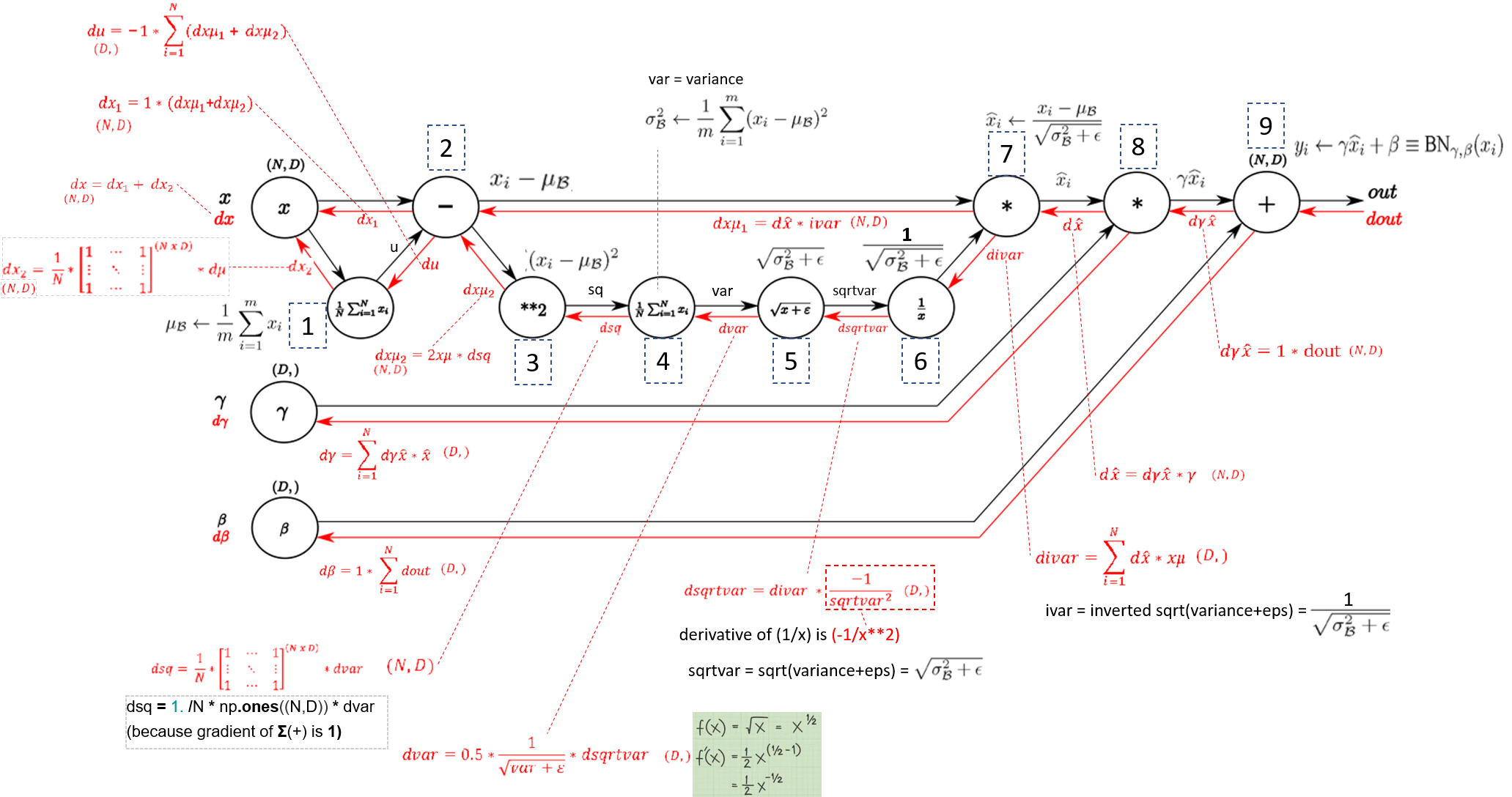
In Python as explained in Understanding the backward pass through Batch Normalization Layer.

enter image description here

enter image description here

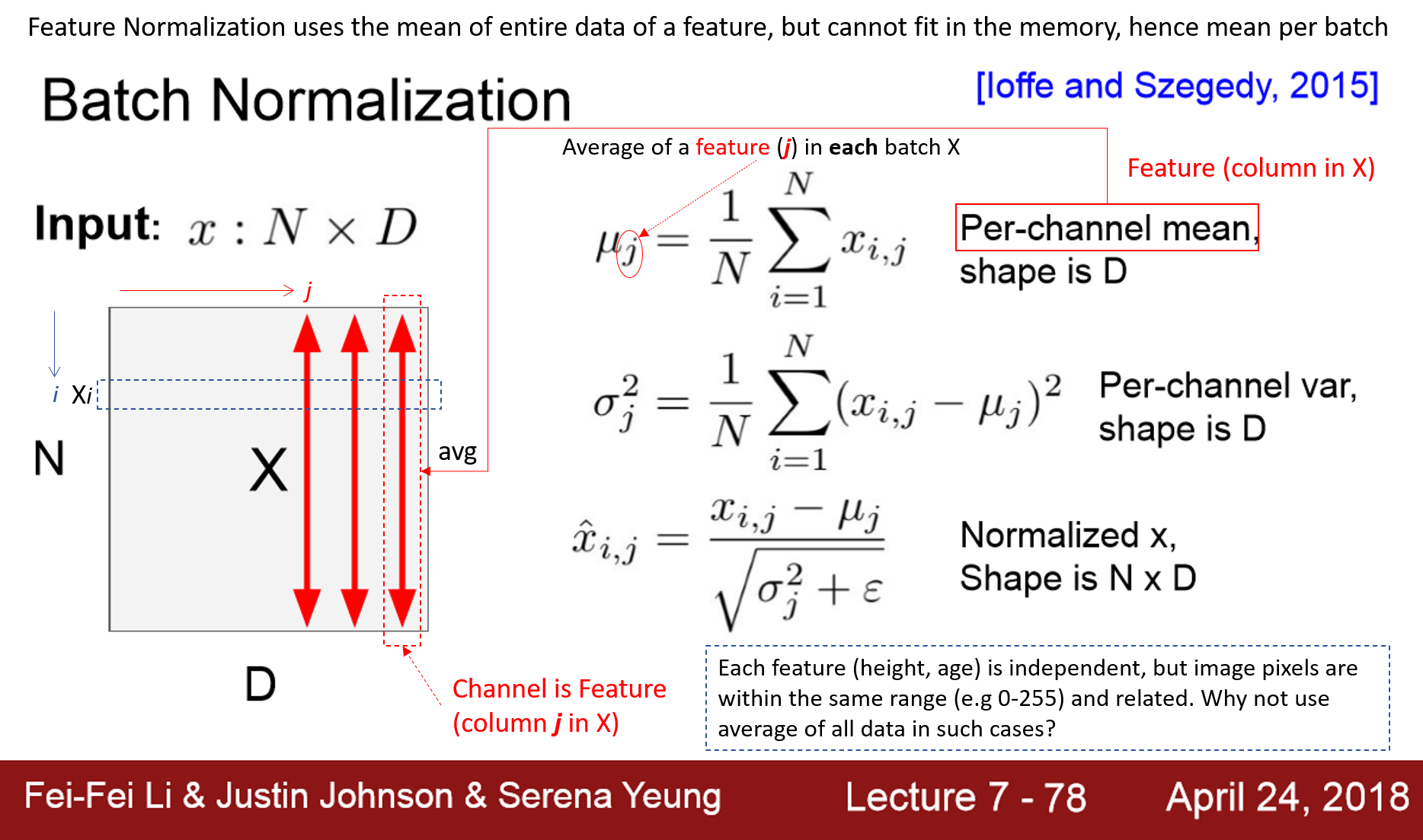
enter image description here

Forward

def batchnorm_forward(x, gamma, beta, eps):

  N, D = x.shape

  #step1: calculate mean
  mu = 1./N * np.sum(x, axis = 0)

  #step2: subtract mean vector of every trainings example
  xmu = x - mu

  #step3: following the lower branch - calculation denominator
  sq = xmu ** 2

  #step4: calculate variance
  var = 1./N * np.sum(sq, axis = 0)

  #step5: add eps for numerical stability, then sqrt
  sqrtvar = np.sqrt(var + eps)

  #step6: invert sqrtwar
  ivar = 1./sqrtvar

  #step7: execute normalization
  xhat = xmu * ivar

  #step8: Nor the two transformation steps
  gammax = gamma * xhat

  #step9
  out = gammax + beta

  #store intermediate
  cache = (xhat,gamma,xmu,ivar,sqrtvar,var,eps)

  return out, cache

Backward

def batchnorm_backward(dout, cache):

  #unfold the variables stored in cache
  xhat,gamma,xmu,ivar,sqrtvar,var,eps = cache

  #get the dimensions of the input/output
  N,D = dout.shape

  #step9
  dbeta = np.sum(dout, axis=0)
  dgammax = dout #not necessary, but more understandable

  #step8
  dgamma = np.sum(dgammax*xhat, axis=0)
  dxhat = dgammax * gamma

  #step7
  divar = np.sum(dxhat*xmu, axis=0)
  dxmu1 = dxhat * ivar

  #step6
  dsqrtvar = -1. /(sqrtvar**2) * divar

  #step5
  dvar = 0.5 * 1. /np.sqrt(var+eps) * dsqrtvar

  #step4
  dsq = 1. /N * np.ones((N,D)) * dvar

  #step3
  dxmu2 = 2 * xmu * dsq

  #step2
  dx1 = (dxmu1 + dxmu2)
  dmu = -1 * np.sum(dxmu1+dxmu2, axis=0)

  #step1
  dx2 = 1. /N * np.ones((N,D)) * dmu

  #step0
  dx = dx1 + dx2

  return dx, dgamma, dbeta

cs231n assignment


def batchnorm_forward(x, gamma, beta, bn_param):
    """
    Forward pass for batch normalization.

    During training the sample mean and (uncorrected) sample variance are
    computed from minibatch statistics and used to normalize the incoming data.
    During training we also keep an exponentially decaying running mean of the
    mean and variance of each feature, and these averages are used to normalize
    data at test-time.

    At each timestep we update the running averages for mean and variance using
    an exponential decay based on the momentum parameter:

    running_mean = momentum * running_mean + (1 - momentum) * sample_mean
    running_var = momentum * running_var + (1 - momentum) * sample_var

    Note that the batch normalization paper suggests a different test-time
    behavior: they compute sample mean and variance for each feature using a
    large number of training images rather than using a running average. For
    this implementation we have chosen to use running averages instead since
    they do not require an additional estimation step; the torch7
    implementation of batch normalization also uses running averages.

    Input:
    - x: Data of shape (N, D)
    - gamma: Scale parameter of shape (D,)
    - beta: Shift paremeter of shape (D,)
    - bn_param: Dictionary with the following keys:
      - mode: 'train' or 'test'; required
      - eps: Constant for numeric stability
      - momentum: Constant for running mean / variance.
      - running_mean: Array of shape (D,) giving running mean of features
      - running_var Array of shape (D,) giving running variance of features

    Returns a tuple of:
    - out: of shape (N, D)
    - cache: A tuple of values needed in the backward pass
    """
    mode = bn_param["mode"]
    eps = bn_param.get("eps", 1e-5)
    momentum = bn_param.get("momentum", 0.9)

    N, D = x.shape
    running_mean = bn_param.get("running_mean", np.zeros(D, dtype=x.dtype))
    running_var = bn_param.get("running_var", np.zeros(D, dtype=x.dtype))

    out, cache = None, None
    if mode == "train":
        #######################################################################
        # TODO: Implement the training-time forward pass for batch norm.      #
        # Use minibatch statistics to compute the mean and variance, use      #
        # these statistics to normalize the incoming data, and scale and      #
        # shift the normalized data using gamma and beta.                     #
        #                                                                     #
        # You should store the output in the variable out. Any intermediates  #
        # that you need for the backward pass should be stored in the cache   #
        # variable.                                                           #
        #                                                                     #
        # You should also use your computed sample mean and variance together #
        # with the momentum variable to update the running mean and running   #
        # variance, storing your result in the running_mean and running_var   #
        # variables.                                                          #
        #                                                                     #
        # Note that though you should be keeping track of the running         #
        # variance, you should normalize the data based on the standard       #
        # deviation (square root of variance) instead!                        #
        # Referencing the original paper (https://arxiv.org/abs/1502.03167)   #
        # might prove to be helpful.                                          #
        #######################################################################
        # *****START OF YOUR CODE (DO NOT DELETE/MODIFY THIS LINE)*****

        #pass
        N = float(N)
        D = float(D)
        x_means = np.sum(x, axis=0) / N                        # shape (1, D)
        x_centered = x - feature_means                         # shape (N, D)
        x_variances = np.sum(np.square(x_centered)) / N        # shape (1, D)
        
        x_normalized = x_centered - np.sqrt(x_variances + eps) # shape (N, D)
        
        running_mean = momentum * running_mean + (1 - momentum) * x_means
        running_var = momentum * running_var + (1 - momentum) * x_variances
        
        out = gamma * x_normalied + beta

        # *****END OF YOUR CODE (DO NOT DELETE/MODIFY THIS LINE)*****
        #######################################################################
        #                           END OF YOUR CODE                          #
        #######################################################################
    elif mode == "test":
        #######################################################################
        # TODO: Implement the test-time forward pass for batch normalization. #
        # Use the running mean and variance to normalize the incoming data,   #
        # then scale and shift the normalized data using gamma and beta.      #
        # Store the result in the out variable.                               #
        #######################################################################
        # *****START OF YOUR CODE (DO NOT DELETE/MODIFY THIS LINE)*****

        pass

        # *****END OF YOUR CODE (DO NOT DELETE/MODIFY THIS LINE)*****
        #######################################################################
        #                          END OF YOUR CODE                           #
        #######################################################################
    else:
        raise ValueError('Invalid forward batchnorm mode "%s"' % mode)

    # Store the updated running means back into bn_param
    bn_param["running_mean"] = running_mean
    bn_param["running_var"] = running_var

    return out, cache


def batchnorm_backward(dout, cache):
    """
    Backward pass for batch normalization.

    For this implementation, you should write out a computation graph for
    batch normalization on paper and propagate gradients backward through
    intermediate nodes.

    Inputs:
    - dout: Upstream derivatives, of shape (N, D)
    - cache: Variable of intermediates from batchnorm_forward.

    Returns a tuple of:
    - dx: Gradient with respect to inputs x, of shape (N, D)
    - dgamma: Gradient with respect to scale parameter gamma, of shape (D,)
    - dbeta: Gradient with respect to shift parameter beta, of shape (D,)
    """
    dx, dgamma, dbeta = None, None, None
    ###########################################################################
    # TODO: Implement the backward pass for batch normalization. Store the    #
    # results in the dx, dgamma, and dbeta variables.                         #
    # Referencing the original paper (https://arxiv.org/abs/1502.03167)       #
    # might prove to be helpful.                                              #
    ###########################################################################
    # *****START OF YOUR CODE (DO NOT DELETE/MODIFY THIS LINE)*****

    pass

    # *****END OF YOUR CODE (DO NOT DELETE/MODIFY THIS LINE)*****
    ###########################################################################
    #                             END OF YOUR CODE                            #
    ###########################################################################

    return dx, dgamma, dbeta
$\endgroup$

Your Answer

By clicking “Post Your Answer”, you agree to our terms of service and acknowledge you have read our privacy policy.

Not the answer you're looking for? Browse other questions tagged or ask your own question.