Characterizing/Fitting Word Count Data into Zipf / Power Law / LogNormal

Question

Using NLTK and Pandas, I was able to process some text files and generate word count data for them, and finally create a histogram describing word frequency.

However, I'm wondering what kind of analysis should I do in order to characterize this distribution. I'm not sure how should I proceed in order to characterize it. I know for a fact that it wouldn't be possible to fit it into a Poisson distribution as the mean is different from the variance.

Any pointers on how can I find out which type of distribution could this data be fit into? Since we're talking about discrete data and looking at the histogram, my initial guesses were Poisson or Negative Binomial. However, mean is different from variance so that would leave me with negative binomial, or binomial.

I tend to think that Negative Binomial is more likely, however I still have to figure out a way to test this assumption.

Answer 1

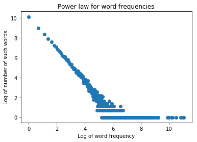
The distribution of word frequencies is often characterized by Zipf's law, which states that it has Pareto distribution $p(k) \sim k^{-s}$, so-called power law.

This power law can be well seen as a straight line on the log-log plot of word counts:

import nltk.corpus
import numpy as np
import matplotlib.pyplot as plt
from collections import Counter
# may need nltk.download() to use Brown corpus
counter_of_words = Counter(nltk.corpus.brown.words())
counter_of_counts = Counter(counter_of_words.values())
word_counts = np.array(list(counter_of_counts.keys()))
freq_of_word_counts = np.array(list(counter_of_counts.values()))
plt.scatter(np.log(word_counts), np.log(freq_of_word_counts))
plt.xlabel('Log of word frequency')
plt.ylabel('Log of number of such words')
plt.title('Power law for word frequencies')
plt.show();

The negated slope of this line (roughly 0.5) corresponds to the parameter $s$ of the Zipf law. You can estimate this value with maximizing likelihood:

def neg_zipf_likelihood(s):
    n = sum(freq_of_word_counts)
    # for each word count, find the probability that a random word has such word count
    probas = word_counts ** (-s) / np.sum(np.arange(1, n+1) **(-s))
    log_likelihood = sum(np.log(probas) * word_counts)
    return -log_likelihood

from scipy.optimize import minimize_scalar
s_best = minimize_scalar(neg_zipf_likelihood, [0.1, 3.0] )
print(s_best.x)

which gives you the value of 0.5366.

If you are still not sure whether you need Zipf's distribution or any other distribution, you can compare log likelihood of your data under different distribution, or choose one using Kolmogorov-Smirnov test.

Answer 2

I have used the example of David Dale for implementing a MLE power law discrete function.

import nltk.corpus
import numpy as np
import matplotlib.pyplot as plt
from collections import Counter
# may need nltk.download() to use Brown corpus
counter_of_words = Counter(nltk.corpus.brown.words())
counter_of_counts = Counter(counter_of_words.values())

# We sort data
counter_of_counts = sorted(counter_of_counts.items(), key=lambda pair: pair[1], reverse=True)
word_counts = np.asarray(counter_of_counts)[:,0]
freq_of_word_counts = np.asarray(counter_of_counts)[:,1]


f,ax = plt.subplots()
ax.scatter(word_counts, freq_of_word_counts, label = "data")
ax.set_xlabel('Word frequency')
ax.set_ylabel('Number of such words')
ax.set_xscale("log")
ax.set_yscale("log")



def loglik(b):  
    # Power law function
    Probabilities = word_counts**(-b)

    # Normalized
    Probabilities = Probabilities/Probabilities.sum()

    # Log Likelihoood
    Lvector = np.log(Probabilities)

    # Multiply the vector by frequencies
    Lvector = np.log(Probabilities) * freq_of_word_counts

    # LL is the sum
    L = Lvector.sum()

    # We want to maximize LogLikelihood or minimize (-1)*LogLikelihood
    return(-L)

s_best = minimize(loglik, [2])
print(s_best)
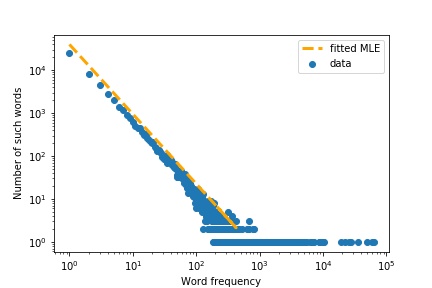
ax.plot(word_counts[0:2*10**2], 4*10**4*word_counts[0:2*10**2]**-s_best.x, '--', color="orange", lw=3, label = "fitted MLE")
ax.legend()

The result give us a slope of 1.62 which visually fits the data very well.

Answer 3

David Dale's answer is a nice demo but unfortunately has a typo. The log likelihood scaling should be by freq_of_word_counts and not word_counts. This is why he gets a clearly invalid slope of -0.5366.

ivangtorre's answer is also nice in that it plots the MLE-fitted distribution. However his answer is also incorrect in that it computes the normalization term of the Zipf distribution in terms of the observed quantities. This is why he also gets an invalid slope of -1.62.

I believe the correct scaling factor is is -1.674. This is approximately the slope of the graph in David Dale's plot and as pointed out by ivangtorre in his comment to David Dale's post ("The slope in your data looks to be 1.66 (10/6).").

The correct calculation is as follows.

from collections import Counter

import matplotlib.pyplot as plt
import nltk
import numpy as np
import scipy as sp

try:
  nltk.corpus.brown.words
except LookupError:
  nltk.download('brown')

counter_of_words = Counter(nltk.corpus.brown.words())
counter_of_counts = Counter(counter_of_words.values())

counter_of_counts = sorted(
    counter_of_counts.items(),
    key=lambda pair: pair[1],
    reverse=True)
word_counts, freq_of_word_counts = np.asarray(counter_of_counts).T


def negloglik_zipf(s, word_counts, freq_of_word_counts):
  # Reference: https://www.johndcook.com/blog/2021/12/11/zeta-zipf-yule/
  log_probs = -s * np.log(word_counts)
  document_length = sum(freq_of_word_counts)
  all_possible_counts = np.arange(1, document_length + 1)
  log_probs -= sp.special.logsumexp(-s * np.log(all_possible_counts))
  return -np.sum(freq_of_word_counts * log_probs)
loss_fn = lambda s: negloglik_zipf(s, word_counts, freq_of_word_counts)
s_best = sp.optimize.minimize_scalar(loss_fn, [0.1, 3.0])
print(s_best)


f, ax = plt.subplots()
ax.scatter(word_counts, freq_of_word_counts, label='data')
ax.set_title('Power law for word frequencies')
ax.set_xlabel('Word frequency')
ax.set_ylabel('Number of such words')
ax.set_xscale('log')
ax.set_yscale('log')

g = np.arange(1, 500)
ax.plot(g, g**(-s_best.x) * max(freq_of_word_counts),
        '--', color='orange', lw=3, label='MLE Zipf')
ax.legend()