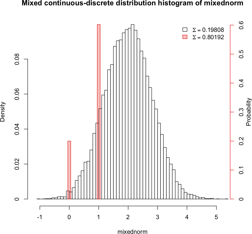
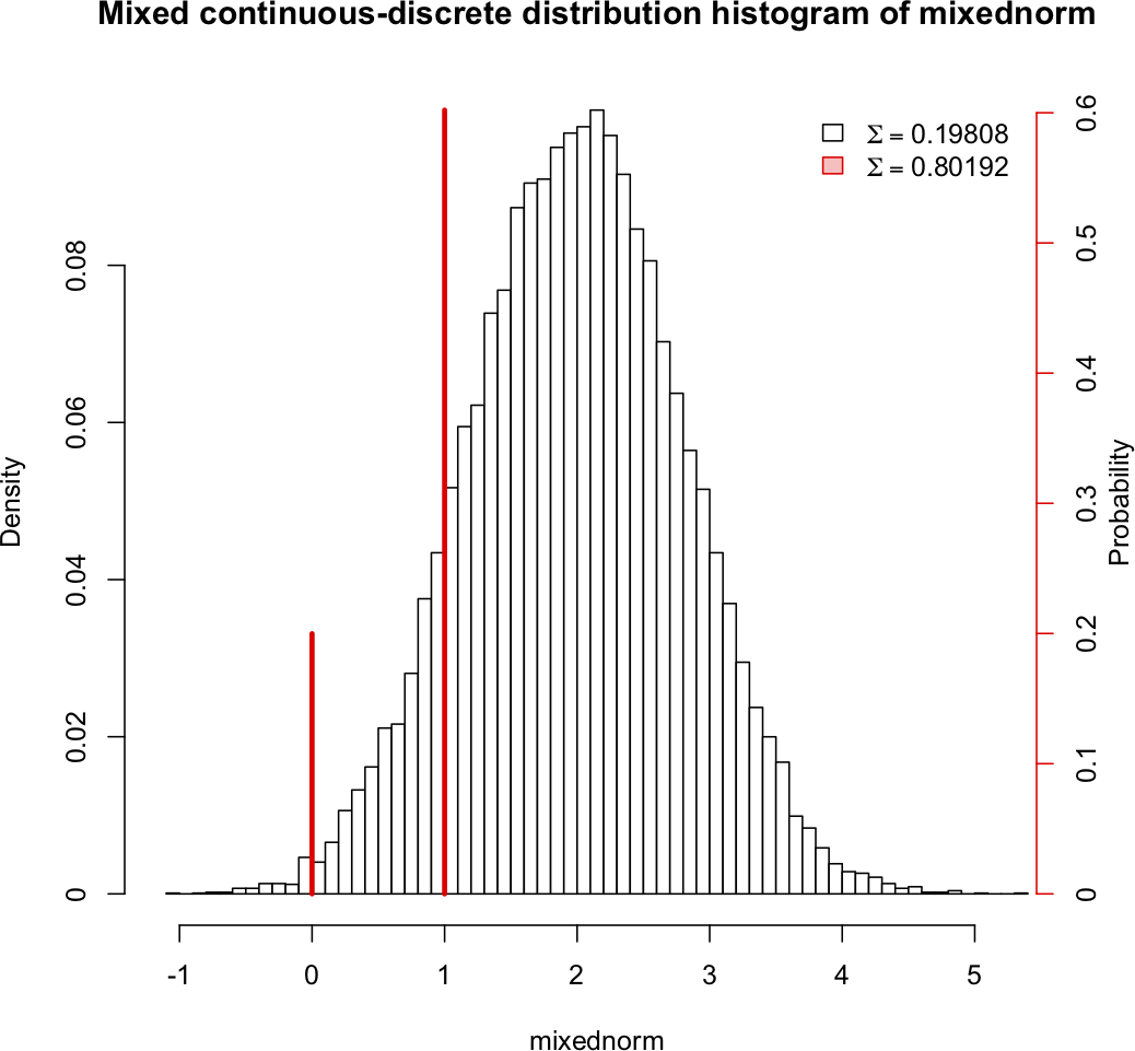
The two are not on the same "scale" (probability is p(x) for the discrete and f(x)dx for the continuous, so p and f are very different things); strictly speaking the way to draw the distribution for a mixed variable would be to draw the cdf.
You could also draw the discrete and continuous parts separately, as you suggest.
I don't think there are any standard names for such a drawing.
Some people draw the two parts on the same plot, but the meaning of the function values is quite different and you get behaviour that people don't usually expect (though it's not at all surprising when you consider it) when you try to deal with discrete and continuous parts together.
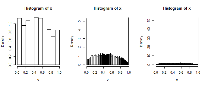
Consider, for example, doing a histogram where you take more bins as you get more data -- then the apparent shape of the histogram changes with sample size. Since judging shape is what people use histograms for, it somewhat defeats the purpose. One of the things you lose by trying to draw them on the same plot is having the histogram "converge" to something you'd like to see (the finite continuous parts disappear down to zero).

Three histograms of a large sample from a 0-1 inflated beta, with different numbers of bins.
None of those plots look much like what you get if you draw the density of the continuous part and then try to mark in the probabilities using the scale on the y-axis (which again is not really appropriate in any case).
While I generally advise against trying to draw both on the same plot, if you do such a thing, you really have to explain very carefully what's going on so people interpret the drawing correctly.
I broke my usual rule when drawing the last plot in this answer:
A model for non-negative data with many zeros: pros and cons of Tweedie GLM
but I did at least explain the problem there. Note that the probability spike at 0 is roughly the same height in each sub-plot even though it looks huge in some and tiny in others - while sometimes it's convenient to break the rule of not putting both on the same plot, one must consider carefully the degree to which you mislead people by doing so. [You often see this done in some fashion with the Tweedie (I've seen it in at least four papers). One example is Figure 1 of Dunn & Smyth (2001)
"Tweedie Family Densities: Methods of Evaluation",
Proceedings of the 16th International Workshop on Statistical Modelling, Odense, Denmark, 2–6 July. (pdf preprint). It's not such a problem if everyone is clear what they're looking at]


