Monte Carlo simulation of integral diverges

Question

If we want to do a simple Monte Carlo evaluation of the expectation of a rv, say X, which is a definite integral, and we find when we evaluate this definite integral analytically that it is infinite.

If this is the case, would we be confident in our Monte Carlo simulation result? I would think not. I think the reason why we would not be confident has to do with L.L.N. but I can't exactly put it into words.

For example, I ran a M.C simulation on a definite integral to find the E[x] like above, and found it has a value between [0,1] instead of being infinite, can anyone explain why this is the case?

Answer 1

The fundamental validation of the Monte Carlo method is the Law of Large Numbers: when $𝔼[X]$ does exist, meaning when $𝔼[|X|]$ is finite, then the empirical average$$\bar{X}_T=\frac{1}{T}\sum_{t=1}^T X_t$$converges almost surely to $𝔼[X]$.

When the expectation $𝔼[X]$ does not exist, meaning$$\int |x|f(x)\text{d}x=+\infty$$there is no guarantee for the empirical average to converge, see e.g. the case of the iid standard Cauchy sequence, when $\bar{X}_T$ remains a standard Cauchy for all $T$'s. But there also exist cases when it converges, as discussed in another XV question:

Counter-examples provided in Wikipedia are

1. $X=\sin(Z)\exp\{Z\}/Z$ when $Z\sim\mathcal{E}xp(1)$, with $\mu=\pi/2$
2. $X=2^Z(-1)^Z/z$ when $Z\sim\mathcal{G}(1/2)$, with $\mu=-\log(2)$
3. $X\sim F(x)$ with $$F(x)=\mathbb{I}_{x\ge e}-\frac{e\mathbb{I}_{x\ge e}}{2x\log(x)}-\frac{e\mathbb{I}_{x\le-e}}{2x\log(-x)}+\frac{\mathbb{I}_{-e\le x\le e}}{2}$$with $\mu=0$

[in the sense that the rv's have no expectation but there exists a limit $\mu$$-$in probability if not a.s.$-$for the sample average $\bar{X}_n$].

See also this quite informative answer on XV.

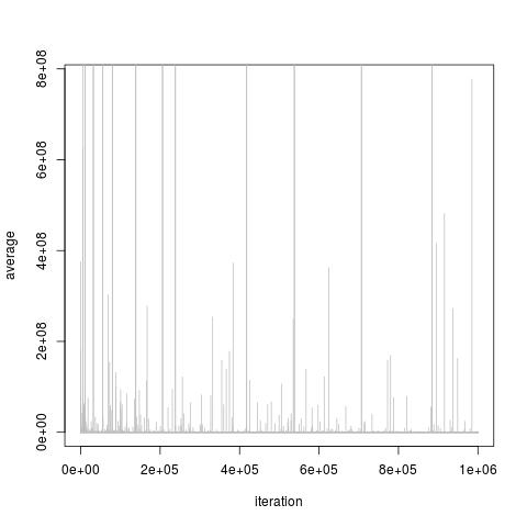
Now, if you take an easily divergent example such as the Pareto $\cal{P}(1/2,4)$ distribution $$f(x)=x^{-3/2}\mathbb{I}_{x>4}$$ simulating this distribution is equivalent to turn a uniform $U$ into $4/U^2$. The mean of the Pareto $\cal{P}(1/2,4)$ distribution is infinite: $$\int_4^\infty x^{-1/2}\text{d}x=+\infty$$But a Monte Carlo experiment does not exhibit a lack of convergence or convergence to $+\infty$, simply that the average can take arbitrarily large values after any number of iterations, as demonstrated on this experiment with 10⁶ simulations, repeated 10² times:

Note also that, in the case of positive rv's like the Pareto $\cal{P}(1/2,4)$ distribution above, $\bar{X}_T$ does not have to converge to infinity if $\mathbb{E}[X]=\infty$. Indeed by Chebychev's inequality, \begin{align*} \mathbb{P}(\bar{X}_T\ge a) &\le \frac{1}{a^\epsilon}\int_{x>a} x^\epsilon \text{d}\mathbb{P}^{\bar{X}_T}(x) \end{align*} which may be finite for $\epsilon>0$ small enough, in which case the rhs probability goes to zero as $a$ goes to infinity.

Answer 2

Running Monte Carlo on undefined value is a common trap when working stable distributions or distributions with fat tails. For instance, suppose you are dealing with Cauchy distribution. You get a bunch of realizations and calculate the mean. The problem is that Cauchy doesn't have a mean, so your result is going to be nonsense.

Here's why. Your Cauchy random numbers are $x_i$, and you calculate the average $\bar x=\frac 1 n\sum_{i=1}^nx_i$. When you have good behaving random numbers, due to CLT the variance of $\bar x$, which is itself a random number is going to decline with sample size increase as $\sigma^2/n$ where $\sigma^2=Var[x_i]$.

With Cauchy distribution and with stable distributions this doesn't happen. The variance will keep growing with sample size. So, the same thing happens in Monte Carlo simulations: you get the finite result for the estimator, but its variance increases as you run more simulations, so your mean becomes less and less certain. Actually, with Cauchy distribution the variance itself is undefined: $\sigma^2=\infty$

My example with Cauchy distribution may feel artificial and forced if you're in social sciences. However, this distribution is known as Lorentzian distribution in physics and is sometimes written in a different parameterization. You run into this thing when dealing with certain spectra. Although it's bell shaped like Gaussian, you fit not the mean and standard deviation, but the center and half-width at half-height. These two are properly defined and can be robustly estimated.