Synopsis
When the predictors are correlated, a quadratic term and an interaction term will carry similar information. This can cause either the quadratic model or the interaction model to be significant; but when both terms are included, because they are so similar neither may be significant. Standard diagnostics for multicollinearity, such as VIF, may fail to detect any of this. Even a diagnostic plot, specifically designed to detect the effect of using a quadratic model in place of interaction, may fail to determine which model is best.
Analysis
The thrust of this analysis, and its main strength, is to characterize situations like that described in the question. With such a characterization available it's then an easy task to simulate data that behave accordingly.
Consider two predictors $X_1$ and $X_2$ (which we will automatically standardize so that each has unit variance in the dataset) and suppose the random response $Y$ is determined by these predictors and their interaction plus independent random error:
$$Y = \beta_1 X_1 + \beta_2 X_2 + \beta_{1,2} X_1 X_2 + \varepsilon.$$
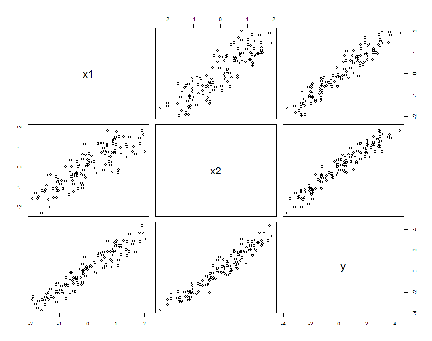
In many cases predictors are correlated. The dataset might look like this:

These sample data were generated with $\beta_1=\beta_2=1$ and $\beta_{1,2}=0.1$. The correlation between $X_1$ and $X_2$ is $0.85$.
This doesn't necessarily mean we are thinking of $X_1$ and $X_2$ as realizations of random variables: it can include the situation where both $X_1$ and $X_2$ are settings in a designed experiment, but for some reason these settings are not orthogonal.
Regardless of how the correlation arises, one good way to describe it is in terms of how much the predictors differ from their average, $X_0 = (X_1+X_2)/2$. These differences will be fairly small (in the sense that their variance is less than $1$); the greater the correlation between $X_1$ and $X_2$, the smaller these differences will be. Writing, then, $X_1 = X_0 + \delta_1$ and $X_2 = X_0 + \delta_2$, we can re-express (say) $X_2$ in terms of $X_1$ as $X_2 = X_1 + (\delta_2-\delta_1)$. Plugging this into the interaction term only, the model is
$$\eqalign{
Y &= \beta_1 X_1+ \beta_2 X_2 + \beta_{1,2}X_1(X_1+ [\delta_2-\delta_1]) + \varepsilon \\
&= (\beta_1 + \beta_{1,2}[\delta_2-\delta_1]) X_1+ \beta_2 X_2 + \beta_{1,2}X_1^2 + \varepsilon
}$$
Provided the values of $\beta_{1,2}[\delta_2-\delta_1]$ vary only a little bit compared to $\beta_1$, we can gather this variation with the true random terms, writing
$$Y = \beta_1 X_1+ \beta_2 X_2 + \beta_{1,2}X_1^2 + \left(\varepsilon +\beta_{1,2}[\delta_2-\delta_1] X_1\right)$$
Thus, if we regress $Y$ against $X_1, X_2$, and $X_1^2$, we will be making an error: the variation in the residuals will depend on $X_1$ (that is, it will be heteroscedastic). This can be seen with a simple variance calculation:
$$\text{var}\left(\varepsilon +\beta_{1,2}[\delta_2-\delta_1] X_1\right) = \text{var}(\varepsilon) + \left[\beta_{1,2}^2\text{var}(\delta_2-\delta_1)\right]X_1^2.$$
However, if the typical variation in $\varepsilon$ substantially exceeds the typical variation in $\beta_{1,2}[\delta_2-\delta_1] X_1$, that heteroscedasticity will be so low as to be undetectable (and should yield a fine model). (As shown below, one way to look for this violation of regression assumptions is to plot the absolute value of the residuals against the absolute value of $X_1$--remembering first to standardize $X_1$ if necessary.) This is the characterization we were seeking.
Remembering that $X_1$ and $X_2$ were assumed to be standardized to unit variance, this implies the variance of $\delta_2-\delta_1$ will be relatively small. To reproduce the observed behavior, then, it should suffice to pick a small absolute value for $\beta_{1,2}$, but make it large enough (or use a large enough dataset) so that it will be significant.
In short, when the predictors are correlated and the interaction is small but not too small, a quadratic term (in either predictor alone) and an interaction term will be individually significant but confounded with each other. Statistical methods alone are unlikely to help us decide which is better to use.
Example
Let's check this out with the sample data by fitting several models. Recall that $\beta_{1,2}$ was set to $0.1$ when simulating these data. Although that is small (the quadratic behavior is not even visible in the previous scatterplots), with $150$ data points we have a chance of detecting it.
First, the quadratic model:
            Estimate Std. Error t value Pr(>|t|)
(Intercept)  0.03363    0.03046   1.104  0.27130
x1           0.92188    0.04081  22.592  < 2e-16 ***
x2           1.05208    0.04085  25.756  < 2e-16 ***
I(x1^2)      0.06776    0.02157   3.141  0.00204 **

Residual standard error: 0.2651 on 146 degrees of freedom
Multiple R-squared: 0.9812, Adjusted R-squared: 0.9808
The quadratic term is significant. Its coefficient, $0.068$, underestimates $\beta_{1,2}=0.1$, but it's of the right size and right sign. As a check for multicollinearity (correlation among the predictors) we compute the variance inflation factors (VIF):
      x1       x2  I(x1^2)
3.531167 3.538512 1.009199
Any value less than $5$ is usually considered just fine. These are not alarming.
Next, the model with an interaction but no quadratic term:
            Estimate Std. Error t value Pr(>|t|)
(Intercept)  0.02887    0.02975    0.97 0.333420
x1           0.93157    0.04036   23.08  < 2e-16 ***
x2           1.04580    0.04039   25.89  < 2e-16 ***
x1:x2        0.08581    0.02451    3.50 0.000617 ***

Residual standard error: 0.2631 on 146 degrees of freedom
Multiple R-squared: 0.9815, Adjusted R-squared: 0.9811

      x1       x2    x1:x2
3.506569 3.512599 1.004566
All the results are similar to the previous ones. Both are about equally good (with a very tiny advantage to the interaction model).
Finally, let's include both the interaction and quadratic terms:
            Estimate Std. Error t value Pr(>|t|)
(Intercept)  0.02572    0.03074   0.837    0.404
x1           0.92911    0.04088  22.729   <2e-16 ***
x2           1.04771    0.04075  25.710   <2e-16 ***
I(x1^2)      0.01677    0.03926   0.427    0.670
x1:x2        0.06973    0.04495   1.551    0.123

Residual standard error: 0.2638 on 145 degrees of freedom
Multiple R-squared: 0.9815, Adjusted R-squared: 0.981

      x1       x2  I(x1^2)    x1:x2
3.577700 3.555465 3.374533 3.359040
Now, neither the quadratic term nor the interaction term are significant, because each is trying to estimate a part of the interaction in the model. Another way to see this is that nothing was gained (in terms of reducing the residual standard error) when adding the quadratic term to the interaction model or when adding the interaction term to the quadratic model. It is noteworthy that the VIFs do not detect this situation: although the fundamental explanation for what we have seen is the slight collinearity between $X_1$ and $X_2$, which induces a collinearity between $X_1^2$ and $X_1 X_2$, neither is large enough to raise flags.
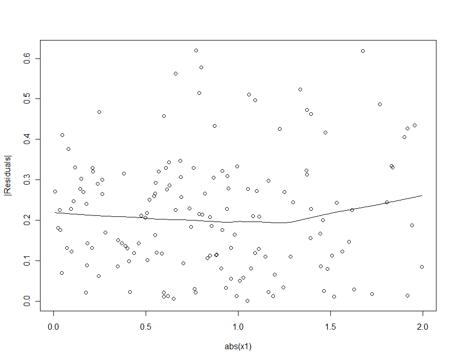
If we had tried to detect the heteroscedasticity in the quadratic model (the first one), we would be disappointed:

In the loess smooth of this scatterplot there is ever so faint a hint that the sizes of the residuals increase with $|X_1|$, but nobody would take this hint seriously.


