2
$\begingroup$

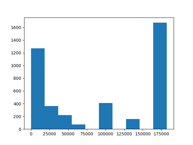
So I was transforming data for machine learning purposes and checking whether I should use the data or log-transform it. In addition to creating histograms I decided to test for normality using scipy.stats.normaltest. The data looks as follows.

NORMAL?

The result of the normality test for this particular data was that the p-value=0.73. Now, I don't claim to be a statistician. However... This does not look like a normal distribution. I tested with a np.random.normal(0, 1, size=1000) and it gave something along the lines of p=0.2 and increasing it to a hundred thousand points gave p=0.6. My data holds ~4000 records.

So I must ask. Have I missed something here? Some of the other vaguely log-normally distributed variables gave p-values of the order 10^-20 after transforming. Does the value of the Chi^2 test need to be incorporated in some manner?

I'm really lost.

Edit:

Running the normaltest on the whole DataFrame gives different results, which adds to the confusion. It gives the same Chi^2 value, but a halved p-value of 0.365...

Edit II

Just for the heck of it, this data gives a similar graph but a p-value of 0.97. What.

>>> a = np.sort(df['col'].values).tolist()[::10]
[0.0001, 0.0001, 0.0001, 0.0001, 0.0001, 0.0001, 0.0001, 0.0001, 0.0001, 0.0001, 0.0001, 0.0001, 0.0001, 0.0001, 0.0001, 0.0001, 0.0001, 0.0001, 0.0001, 0.0001, 0.0001, 0.0001, 0.0001, 0.0001, 0.0001, 0.0001, 0.0001, 0.0001, 0.0001, 0.0001, 0.0001, 0.0001, 0.0001, 0.0001, 0.0001, 0.0001, 0.0001, 0.0001, 0.0001, 0.0001, 0.0001, 0.0001, 0.0001, 0.0001, 0.0001, 0.0001, 0.0001, 0.0001, 0.0001, 0.0001, 0.0001, 0.0001, 0.0001, 0.0001, 0.0001, 0.0001, 0.0001, 0.0001, 0.0001, 0.0001, 0.0001, 0.0001, 0.0001, 0.0001, 0.0001, 0.0001, 0.0001, 0.0001, 0.0001, 0.0001, 0.0001, 0.0001, 0.0001, 0.0001, 0.0001, 0.0001, 0.0001, 0.0001, 0.0001, 0.0001, 0.0001, 0.0001, 0.0001, 0.0001, 0.0001, 0.0001, 0.0001, 0.0001, 0.0001, 0.0001, 0.0001, 0.0001, 0.0001, 0.0001, 0.0001, 0.0001, 0.0001, 0.0001, 0.0001, 0.0001, 0.0001, 0.0001, 0.0001, 0.0001, 0.0001, 0.0001, 0.0001, 0.0001, 0.0001, 0.0001, 0.0001, 0.0001, 0.0001, 0.0001, 0.0001, 0.0001, 0.0001, 0.0001, 0.0001, 0.0001, 0.0001, 0.0001, 0.0001, 0.0001, 0.0001, 0.0001, 0.0001, 0.0001, 0.1622, 0.1622, 0.1622, 0.1622, 0.1622, 0.1622, 0.1622, 0.1622, 0.1622, 0.1687, 0.1687, 0.1729, 0.1729, 0.1729, 0.1729, 0.1729, 0.1729, 0.1729, 0.1729, 0.1729, 0.1729, 0.1729, 0.1729, 0.1729, 0.1729, 0.1729, 0.1729, 0.1729, 0.1729, 0.1729, 0.1729, 0.1729, 0.1729, 0.1729, 0.1729, 0.1729, 0.2005, 0.2216, 0.2216, 0.2498, 0.2498, 0.2498, 0.2498, 0.2498, 0.2498, 0.2498, 0.2498, 0.2498, 0.2498, 0.2498, 0.2498, 0.2498, 0.2498, 0.2498, 0.2498, 0.2498, 0.2498, 0.2498, 0.3143, 0.3143, 0.3143, 0.3143, 0.3143, 0.3143, 0.3143, 0.48, 0.4854, 0.4854, 0.4854, 0.4854, 0.4854, 0.4854, 0.4854, 0.5078, 0.5078, 0.5078, 0.5078, 0.5078, 0.5078, 0.5078, 0.5078, 0.5078, 0.5078, 0.5078, 0.5078, 0.5078, 0.5078, 0.5078, 0.5078, 0.5078, 0.5328, 0.5328, 0.5328, 0.5328, 0.5328, 0.5328, 0.5328, 0.5328, 0.5328, 0.5328, 0.5328, 0.5328, 0.5328, 0.5328, 0.5328, 0.5328, 0.6496, 0.6496, 0.6496, 0.6496, 0.6496, 0.6496, 0.6496, 0.6496, 0.6496, 0.6496, 0.6496, 0.6496, 0.6496, 0.6496, 0.6496, 0.6496, 0.9119, 0.9119, 0.9119, 0.9119, 0.9119, 0.9119, 0.9119, 0.9119, 0.9119, 0.9119, 0.9119, 0.9119, 0.9119, 0.9119, 0.9119, 0.9119, 0.9119, 0.9119, 0.9119, 0.9119, 0.9119, 0.9119, 0.9119, 0.9119, 0.9119, 0.9119, 0.9119, 0.9119, 0.9119, 0.9119, 0.9119, 0.9119, 0.9119, 0.9119, 0.9119, 0.9119, 0.9119, 0.9119, 0.9119, 0.9119, 0.9119, 0.9119, 0.9119, 0.9119, 0.9119, 0.9119, 0.9119, 0.9119, 0.9119, 0.9119, 0.9119, 0.9119, 0.9119, 0.9119, 0.9119, 0.9119, 0.9119, 0.9119, 0.9119, 0.9119, 0.9119, 0.9119, 0.9119, 0.9119, 0.9119, 0.9119, 0.9119, 0.9119, 0.9119, 0.9119, 0.9119, 0.9119, 0.9119, 0.9119, 0.9119, 0.9119, 0.9119, 0.9119, 0.9119, 0.9119, 0.9119, 0.9119, 0.9119, 0.9119, 0.9119, 0.9119, 0.9119, 0.9119, 0.9119, 0.9119, 0.9119, 0.9119, 0.9119, 0.9119, 0.9119, 0.9119, 0.9119, 0.9119, 0.9119, 0.9119, 0.9119, 0.9119, 0.9119, 0.9119, 0.9119, 0.9119, 0.9119, 0.9119, 0.9119, 0.9119, 0.9119, 0.9119, 0.9119, 0.9119, 0.9119, 0.9119, 0.9119, 0.9119, 0.9119, 0.9119, 0.9119, 0.9119, 0.9119, 0.9119, 0.9119, 0.9119, 0.9119, 0.9119, 0.9119, 0.9119, 0.9119, 0.9119, 0.9119, 0.9119, 0.9119, 0.9119, 0.9119, 0.9119, 0.9119, 0.9119, 0.9119, 0.9119, 0.9119, 0.9119, 0.9119, 0.9119, 0.9119, 0.9119, 0.9119, 0.9119, 0.9119, 0.9119, 0.9119, 0.9119, 0.9119, 0.9119, 0.912, 0.912, 0.912, 0.912, 0.912, 0.912, 0.912, 0.912, 0.912, 0.912, 0.912]

>>> from scipy.stats import normaltest
>>> normaltest(a)
NormaltestResult(statistic=0.05292848970575527, pvalue=0.9738828645381232)

>>> from matplotlib import pyplot as plt
>>> plt.hist(a) # Results in a similar graph to above
$\endgroup$
7
  • 1
    $\begingroup$ I suspect you might be mis-applying the test: assuming these bars represent counts of data plotted on the horizontal axis, there's no way any test of Normality will fail to reject that hypothesis. However, a log transformation won't cure that problem. Thus, you might be asking a fruitless question in the first place. $\endgroup$
    – whuber
    Commented Jun 29, 2018 at 13:20
  • $\begingroup$ @whuber I'm not saying this was the data I applied the log transform to. Yes they represent the counts. It's a very simple way I'm calling the function. I have a column inside a dataframe with all valid values and the normality test function takes one input. $\endgroup$
    – Felix
    Commented Jun 29, 2018 at 13:22
  • 1
    $\begingroup$ But that's exactly what you are saying! If these aren't the data you are concerned about, then why are you displaying this plot?? Please clarify how you are applying the normality test. Give a small reproducible example. $\endgroup$
    – whuber
    Commented Jun 29, 2018 at 13:31
  • 1
    $\begingroup$ Yes: that's precisely how such a test should behave. With large amounts of data, it's almost impossible for any real dataset to look normal, so a decent test will detect the (tiny) departures from normality. That's one of many reasons why your line of inquiry seems to be of little value. $\endgroup$
    – whuber
    Commented Jun 29, 2018 at 13:35
  • 1
    $\begingroup$ Here's a simpler way to produce an essentially-equivalent dataset: np.hstack([np.full(c, i) for i, c in enumerate([128, 0, 58, 7, 0, 41, 16, 0, 0, 167])]), which just scales everything up and rounds. Either the skewness and kurtosis tests used here are surprisingly bad in this case, or there's a bug in scipy.stats; it seems that you're calling the function correctly. $\endgroup$
    – Danica
    Commented Jun 29, 2018 at 13:49

2 Answers 2

2
$\begingroup$

Unfortunately, there's a bug in scipy.stats.normaltest, specifically in scipy.stats.kurtosistest (Scipy 1.1.0). The data are clearly non-normal, and numerous tests correctly indicate that (ps<.05, see examples in R below). I've reported the bug.

Code and Details:

library(moments)
library(nortest)
x=c(0.0001, 0.0001, 0.0001, 0.0001, 0.0001, 0.0001, 0.0001, 0.0001, 0.0001, 0.0001, 0.0001, 0.0001, 0.0001, 0.0001, 0.0001, 0.0001, 0.0001, 0.0001, 0.0001, 0.0001, 0.0001, 0.0001, 0.0001, 0.0001, 0.0001, 0.0001, 0.0001, 0.0001, 0.0001, 0.0001, 0.0001, 0.0001, 0.0001, 0.0001, 0.0001, 0.0001, 0.0001, 0.0001, 0.0001, 0.0001, 0.0001, 0.0001, 0.0001, 0.0001, 0.0001, 0.0001, 0.0001, 0.0001, 0.0001, 0.0001, 0.0001, 0.0001, 0.0001, 0.0001, 0.0001, 0.0001, 0.0001, 0.0001, 0.0001, 0.0001, 0.0001, 0.0001, 0.0001, 0.0001, 0.0001, 0.0001, 0.0001, 0.0001, 0.0001, 0.0001, 0.0001, 0.0001, 0.0001, 0.0001, 0.0001, 0.0001, 0.0001, 0.0001, 0.0001, 0.0001, 0.0001, 0.0001, 0.0001, 0.0001, 0.0001, 0.0001, 0.0001, 0.0001, 0.0001, 0.0001, 0.0001, 0.0001, 0.0001, 0.0001, 0.0001, 0.0001, 0.0001, 0.0001, 0.0001, 0.0001, 0.0001, 0.0001, 0.0001, 0.0001, 0.0001, 0.0001, 0.0001, 0.0001, 0.0001, 0.0001, 0.0001, 0.0001, 0.0001, 0.0001, 0.0001, 0.0001, 0.0001, 0.0001, 0.0001, 0.0001, 0.0001, 0.0001, 0.0001, 0.0001, 0.0001, 0.0001, 0.0001, 0.0001, 0.1622, 0.1622, 0.1622, 0.1622, 0.1622, 0.1622, 0.1622, 0.1622, 0.1622, 0.1687, 0.1687, 0.1729, 0.1729, 0.1729, 0.1729, 0.1729, 0.1729, 0.1729, 0.1729, 0.1729, 0.1729, 0.1729, 0.1729, 0.1729, 0.1729, 0.1729, 0.1729, 0.1729, 0.1729, 0.1729, 0.1729, 0.1729, 0.1729, 0.1729, 0.1729, 0.1729, 0.2005, 0.2216, 0.2216, 0.2498, 0.2498, 0.2498, 0.2498, 0.2498, 0.2498, 0.2498, 0.2498, 0.2498, 0.2498, 0.2498, 0.2498, 0.2498, 0.2498, 0.2498, 0.2498, 0.2498, 0.2498, 0.2498, 0.3143, 0.3143, 0.3143, 0.3143, 0.3143, 0.3143, 0.3143, 0.48, 0.4854, 0.4854, 0.4854, 0.4854, 0.4854, 0.4854, 0.4854, 0.5078, 0.5078, 0.5078, 0.5078, 0.5078, 0.5078, 0.5078, 0.5078, 0.5078, 0.5078, 0.5078, 0.5078, 0.5078, 0.5078, 0.5078, 0.5078, 0.5078, 0.5328, 0.5328, 0.5328, 0.5328, 0.5328, 0.5328, 0.5328, 0.5328, 0.5328, 0.5328, 0.5328, 0.5328, 0.5328, 0.5328, 0.5328, 0.5328, 0.6496, 0.6496, 0.6496, 0.6496, 0.6496, 0.6496, 0.6496, 0.6496, 0.6496, 0.6496, 0.6496, 0.6496, 0.6496, 0.6496, 0.6496, 0.6496, 0.9119, 0.9119, 0.9119, 0.9119, 0.9119, 0.9119, 0.9119, 0.9119, 0.9119, 0.9119, 0.9119, 0.9119, 0.9119, 0.9119, 0.9119, 0.9119, 0.9119, 0.9119, 0.9119, 0.9119, 0.9119, 0.9119, 0.9119, 0.9119, 0.9119, 0.9119, 0.9119, 0.9119, 0.9119, 0.9119, 0.9119, 0.9119, 0.9119, 0.9119, 0.9119, 0.9119, 0.9119, 0.9119, 0.9119, 0.9119, 0.9119, 0.9119, 0.9119, 0.9119, 0.9119, 0.9119, 0.9119, 0.9119, 0.9119, 0.9119, 0.9119, 0.9119, 0.9119, 0.9119, 0.9119, 0.9119, 0.9119, 0.9119, 0.9119, 0.9119, 0.9119, 0.9119, 0.9119, 0.9119, 0.9119, 0.9119, 0.9119, 0.9119, 0.9119, 0.9119, 0.9119, 0.9119, 0.9119, 0.9119, 0.9119, 0.9119, 0.9119, 0.9119, 0.9119, 0.9119, 0.9119, 0.9119, 0.9119, 0.9119, 0.9119, 0.9119, 0.9119, 0.9119, 0.9119, 0.9119, 0.9119, 0.9119, 0.9119, 0.9119, 0.9119, 0.9119, 0.9119, 0.9119, 0.9119, 0.9119, 0.9119, 0.9119, 0.9119, 0.9119, 0.9119, 0.9119, 0.9119, 0.9119, 0.9119, 0.9119, 0.9119, 0.9119, 0.9119, 0.9119, 0.9119, 0.9119, 0.9119, 0.9119, 0.9119, 0.9119, 0.9119, 0.9119, 0.9119, 0.9119, 0.9119, 0.9119, 0.9119, 0.9119, 0.9119, 0.9119, 0.9119, 0.9119, 0.9119, 0.9119, 0.9119, 0.9119, 0.9119, 0.9119, 0.9119, 0.9119, 0.9119, 0.9119, 0.9119, 0.9119, 0.9119, 0.9119, 0.9119, 0.9119, 0.9119, 0.9119, 0.9119, 0.9119, 0.9119, 0.9119, 0.9119, 0.9119, 0.912, 0.912, 0.912, 0.912, 0.912, 0.912, 0.912, 0.912, 0.912, 0.912, 0.912)

pList <- list()
pList$ShapiroWilk <- shapiro.test(x)$p.value
pList$ShapiroFrancia <- sf.test(x)$p.value
pList$AndersonDarling <- ad.test(x)$p.value
pList$KolmSmirLill <- lillie.test(x)$p.value
pList$PearsonChiSq <- pearson.test(x)$p.value
pList

P-values:

Shapiro-Wilk 1.572961e-23

Shapiro-Francia 2.64774e-20

Anderson-Darling 3.7e-24

Kolmogorov-Smirnov (Lilliefors version) 9.468351e-83

Pearson Chi Squared 0

$\endgroup$
7
  • 1
    $\begingroup$ I now suspect that the Python function is the real problem. I programmed the D'Agostino omnibus test by hand in R, and it gave a p of approximately 0. I verified the R function's accuracy using the D'Agostino et al. example dataset (1990, pg. 138). This may take a while, but I'll try to fix the post.. $\endgroup$
    – Anthony
    Commented Jul 12, 2018 at 18:18
  • 1
    $\begingroup$ Results should be z.skew=-0.2300619, z.kurt=46.98108, chisq= 2207.275, and p=0. There is a part of the formula that's prone to computation errors. Eq 19 in ohio.edu/plantbio/staff/mccarthy/quantmet/D'Agostino.pdf involves a cube-root of a negative number (negative for the dataset in this question), and that tripped up R's default exponent function, so maybe the same issue happens in Python? $\endgroup$
    – Anthony
    Commented Jul 12, 2018 at 18:25
  • 1
    $\begingroup$ The bug is definitely in scipy.stats.kurtosistest located in lines of code attempting to replace negative numbers prior to taking the cube-root. $\endgroup$
    – Anthony
    Commented Jul 13, 2018 at 21:08
  • 1
    $\begingroup$ I've updated it, and reported the bug: github.com/scipy/scipy/issues/9033. I'm a Python noob, so maybe someone who's more familiar can come up with a better solution that what I've proposed. $\endgroup$
    – Anthony
    Commented Jul 14, 2018 at 17:07
  • $\begingroup$ Wow, awesome that the question generated such attention! $\endgroup$
    – Felix
    Commented Jul 15, 2018 at 20:36
1
$\begingroup$

Tha accepted answer from @Anthony makes the main point: your data have tickled a bug in the software you used.

This is a bundle of extra comments using the sample given in Edit II as a sandbox.

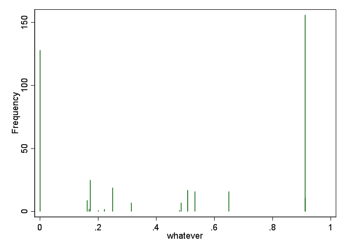
As in the distribution histogram shown in the question for other data, you have a spiky, roughly U-shaped distribution. A logarithmic transformation will not help with such a distribution. It will just make it look and be a worse fit to a normal. The spikes will remain spikes. Here is a graph of the distribution.

enter image description here

There should be a story behind the repeated values: in a sample of 417, you have only a small number of distinct values.

   whatever |      Freq.     Percent        Cum.
------------+-----------------------------------
      .0001 |        128       30.70       30.70
      .1622 |          9        2.16       32.85
      .1687 |          2        0.48       33.33
      .1729 |         25        6.00       39.33
      .2005 |          1        0.24       39.57
      .2216 |          2        0.48       40.05
      .2498 |         19        4.56       44.60
      .3143 |          7        1.68       46.28
        .48 |          1        0.24       46.52
      .4854 |          7        1.68       48.20
      .5078 |         17        4.08       52.28
      .5328 |         16        3.84       56.12
      .6496 |         16        3.84       59.95
      .9119 |        156       37.41       97.36
       .912 |         11        2.64      100.00
------------+-----------------------------------
      Total |        417      100.00

That aside, for these data I get the following results for moment-based statistics in Stata. The definitions used (on which a Gaussian/normal would have skewness 0 and kurtosis 3) are documented on p.9 of this section in the Stata manuals.

Other formulas exist but for this sample size they shouldn't make that much difference.

 ----------------------------------------------------------
  n = 417 |       mean          SD    skewness    kurtosis
----------+-----------------------------------------------
 whatever |      0.473       0.398      -0.027       1.243
----------------------------------------------------------

Some people like to work with so-called excess kurtosis, subtracting 3. Here that would be $−$1.757.

In terms of kurtosis the example data here are clearly non-normal. Any test based on skewness and kurtosis should therefore reject a null of normality. For context, minimum possible kurtosis is 1 (excess kurtosis $−$2); that minimum is attainable if half the data are equal to a maximum and half equal to a minimum (e.g. probability of 0 and of 1 both 0.5). Kurtosis just above 1 is expected for a U-shaped distribution, as here.

How best to treat such data depends on knowing more about how they were produced and your goals.

$\endgroup$
3
  • $\begingroup$ Yep, thanks, although the question wasn't really on whether I should use the log transform or not. But I appreciate it. The fact that the data contained equal values was a result of a round operation - purely for not sharing the real data. That's also why the data was only apx. a tenth of the original size of the histogram. $\endgroup$
    – Felix
    Commented Jul 15, 2018 at 20:34
  • $\begingroup$ Glad it helped. Given this comment, I have to wonder why you started "So I was transforming data for machine learning purposes and checking whether I should use the data or log-transform it." $\endgroup$
    – Nick Cox
    Commented Jul 16, 2018 at 6:59
  • $\begingroup$ Yeah, I guess it was unnecessary, but I felt like giving at least some context for the normality test. $\endgroup$
    – Felix
    Commented Jul 16, 2018 at 7:42

Your Answer

By clicking “Post Your Answer”, you agree to our terms of service and acknowledge you have read our privacy policy.

Not the answer you're looking for? Browse other questions tagged or ask your own question.