ARIMA Model Stage 3 (Residual Diagnostic) - Is the residual a white noise?

Question

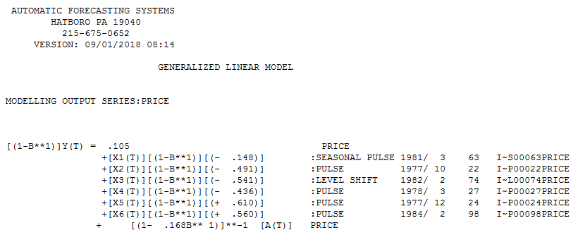
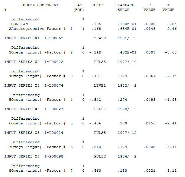
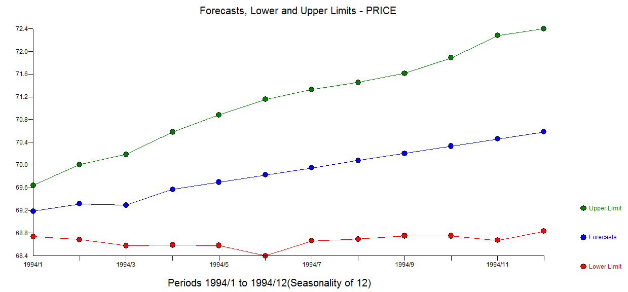
Work Done: I have a monthly time-series data (Consumer Price Index) from 1976 to 1993. I performed first differencing and log transformation to detrend it, also, Augmented Dickey-Fuller Test has confirmed that it is stationary. Then, I use the Automatic ARIMA Forecasting feature in EVIEWS. It suggests that an ARIMA (8,1,8) model is appropriate (with the lowest AIC).

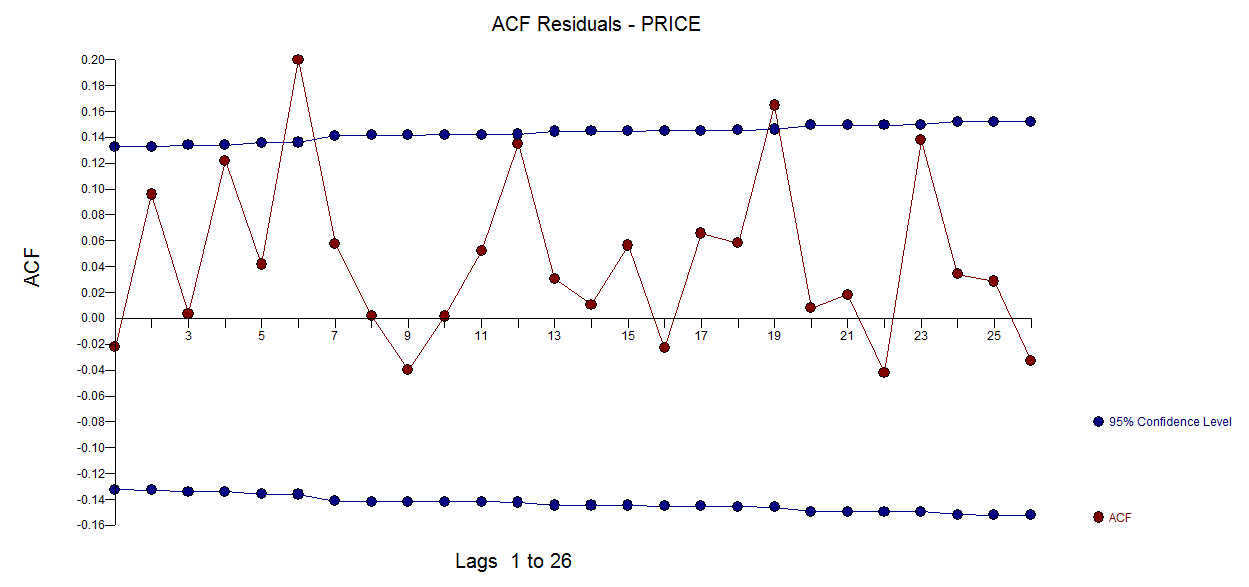
Problem: When i did the residual diagnostic with correlogram to confirm that residual is a white noise. Correlogram shows that, all spikes are within the confidence boundary; however, the p-values shown was lesser than 0.05.

Can I conclude that residual is a white noise? Since all spikes are within the confidence boundary.

Year CPI 
1976 Jan 42.5 
1976 Feb 42.49 
1976 March 41.95 
1976 Apr 41.54 
1976 May 41.71 
1976 June 41.49 
1976 July 41.46 
1976 August 41.41 
1976 Sep 41.33 
1976 October 41.29 
1976 November 41.53 
1976 December 41.86 
1977 Jan 42.42 
1977 Feb 42.7 
1977 March 42.41 
1977 Apr 42.06 
1977 May 42.39 
1977 June 42.55 
1977 July 42.98 
1977 August 43.62 
1977 Sep 43.91 
1977 October 43.29 
1977 November 43.65 
1977 December 44.54 
1978 Jan 44.27 
1978 Feb 44.57 
1978 March 43.98 
1978 Apr 44.24 
1978 May 44.39 
1978 June 44.5 
1978 July 45.03
1978 August 45.24
1978 Sep 45.32
1978 October 45.15
1978 November 45.42
1978 December 45.39
1979 Jan 45.42
1979 Feb 45.27
1979 March 45.13
1979 Apr 45.33
1979 May 45.66
1979 June 45.78
1979 July 46.35
1979 August 47.18
1979 Sep 47.92
1979 October 47.93
1979 November 48.34
1979 December 48.71
1980 Jan 48.76
1980 Feb 49.53
1980 March 50.05
1980 Apr 50.27
1980 May 50.24
1980 June 50.38
1980 July 50.82
1980 August 51.2
1980 Sep 51.08
1980 October 51.25
1980 November 51.58
1980 December 51.63
1981 Jan 51.78
1981 Feb 52.4
1981 March 52.52
1981 Apr 53.58
1981 May 54.27
1981 June 54.64
1981 July 55.46
1981 August 56.    19
1981 Sep 56.09
1981 October 56.11
1981 November 56.48
1981 December 56.97
1982 Jan 57.53
1982 Feb 57.09
1982 March 56.48
1982 Apr 56.5
1982 May 56.54
1982 June 56.69
1982 July 56.54
1982 August 56.77
1982 Sep 56.86
1982 October 56.71
1982 November 57.06
1982 December 57.44
1983 Jan 57.26
1983 Feb 57.37
1983 March 57.31
1983 Apr 57.24
1983 May 57.44
1983 June 57.07
1983 July 57.28
1983 August 57.32
1983 Sep 57.53
1983 October 57.41
1983 November 57.94
1983 December 58.1
1984 Jan 58.68
1984 Feb 59.46
1984 March 58.87
1984 Apr 58.88
1984 May 58.83
1984 June 58.99
1984 July 59.16
1984 August 59.3
1984 Sep 58.9
1984 October 58.87
1984 November 58.65
1984 December 58.63
1985 Jan 58.89
1985 Feb 59.18
1985 March 59.34
1985 Apr 59.22
1985 May 59.21
1985 June 59.36
1985 July 59.56
1985 August 59.63
1985 Sep 59.15
1985 October 59.14
1985 November 58.99
1985 December 59.03
1986 Jan 59
1986 Feb 58.85
1986 March 58.68
1986 Apr 58.38
1986 May 58.34
1986 June 58.25
1986 July 58.16
1986 August 58.13
1986 Sep 58.37
1986 October 58.35
1986 November 58.17
1986 December 58.22
1987 Jan 58.59
1987 Feb 58.22
1987 March 58.22
1987 Apr 58.42
1987 May 58.58
1987 June 58.61
1987 July 58.85
1987 August 58.93
1987 Sep 58.89
1987 October 58.88
1987 November 58.98
1987 December 59.11
1988 Jan 59.02
1988 Feb 59.47
1988 March 59.32
1988 Apr 59.34
1988 May 59.53
1988 June 59.46
1988 July 59.81
1988 August 59.78
1988 Sep 59.84
1988 October 59.71
1988 November 59.79
1988 December 59.94
1989 Jan 59.91
1989 Feb 60.07
1989 March 60.01
1989 Apr 60.35
1989 May 60.78
1989 June 61.06
1989 July 61.23
1989 August 61.31
1989 Sep 61.3
1989 October 61.61
1989 November 61.85
1989 December 61.92
1990 Jan 62.27
1990 Feb 62.39
1990 March 62.21
1990 Apr 62.56
1990 May 62.72
1990 June 62.81
1990 July 62.84
1990 August 63.06
1990 Sep 63.49
1990 October 64
1990 November 63.98
1990 December 64.29
1991 Jan 64.35
1991 Feb 64.88
1991 March 64.57
1991 Apr 64.9
1991 May 65.11
1991 June 65.27
1991 July 65.35
1991 August 65.51
1991 Sep 65.48
1991 October 65.51
1991 November 65.61
1991 December 66.13
1992 Jan 66.13
1992 Feb 66.05
1992 March 65.93
1992 Apr 66.34
1992 May 66.69
1992 June 66.69
1992 July 66.98
1992 August 66.86
1992 Sep 66.91
1992 October 67.07
1992 November 67.26
1992 December 67.32
1993 Jan 67.83
1993 Feb 67.52
1993 March 67.68
1993 Apr 67.88
1993 May 68.07
1993 June 68.09
1993 July 68.42
1993 August 68.31
1993 Sep 68.35
1993 October 68.59
1993 November 68.8
1993 December 69.04

Answer 1

Not necessarily as untreated pulses , level shifts , seasonal pulses or local time trends can severely downwards bias the acf of the model errors leading to an incorrect conclusion that the error process is white noise .

This erroneous conclusion can also be reached if the model parameters or model error variance is not homogeneous through time.

If you post your data I will try to help you further.

Arima modelling is a sequence of self-checking proceedures designed to extract a minimally sufficient signal and a companion noise process free of evidented structure. Your data (216 monthly values) can be easily described by a (1,1,0) arima structure , 4 pulses ( periods 22.24.27 and 98 ) , 1 intercept change at period 74 , 1 seasonal pulse starting at period 63 (1981/3) and 1 error variance change (down) at period 128 culminating in a GLS model.

The model is here and here

Arima models like you describe (8,1,8) are artifacts from an incomplete analysis and are fundamentally laughable. The reason EVIEWS fails is because it does not deal with the model in a holistic manner. See my comment and other threads in response to How to determine order of sarima?

Power transforms do not detrend and should only be employed under certain conditions When (and why) should you take the log of a distribution (of numbers)?.

The acf of the model residuals is here

and forecasts with confidence limits are here . using monte-carlo simulation (bo0tstrap) where future anomalies are explicitely allowed for.

Finally the confidence limits around acf/pacf are VERY VERY VERY approximate as they are purely based on the sample size (+/- t/sqrt(216 where t is the normal deviate) and should not be over-believed.

Another way to answer this question .. is for you to post your residuals and to see if model structure can be found/verified.