Uniform distribution with Gaussian Priors

Question

Let's say i've got a uniform distribution defined as follows $$X \sim U[\min (\theta_1,\theta_2),\max (\theta_1,\theta_2)]$$ I've also got that $\theta_1,\theta_2$ are i.i.d zero-mean normal distributions with variance $\sigma^2$. i.e. $$\theta_k\sim \mathcal{N}(0,\sigma^2) \qquad k \in \lbrace 1,2 \rbrace$$

Question: What is the distribution of $X$, i.e. $f_X(x)$ ?

Efforts: We know that $$f_X(x) = \int\limits f_{X \vert \theta_1,\theta_2}(x \vert \theta_1,\theta_2) f(\theta_1,\theta_2) d\theta_1 d\theta_2$$ Since $\theta_1,\theta_2$ are normal i.i.d, we can say $$f_X(x) = \int\limits f_{X \vert \theta_1,\theta_2}(x \vert \theta_1,\theta_2) \phi_{\sigma}(\theta_1)\phi_{\sigma}(\theta_2) d\theta_1 d\theta_2$$ where $f_{X \vert \theta_1,\theta_2}$ is the uniform distribution bounded by $\theta_1,\theta_2$ and $\phi_{\sigma}(x)$ is the Gaussian PDF with zero mean and standard deviation $\sigma$. This integral is really messy to solve. Does someone know a roundabout of this ?

Spoiler: Through simulations, i've seen that $X$ is normally distributed with zero mean and standard deviation $\sim 0.8166\sigma$.

Answer 1

Let $\psi_1$, $\psi_2$ be order statistics of $N(0,\sigma^2)$.

I used them instead of $\theta$s, then $\psi_1 \leq x\leq\psi_2$ and

$$f_X(x)=\int^\infty_x \int^x_{-\infty}\frac{1}{\psi_2-\psi_1} 2! \phi_{\sigma}(\psi_1)\phi_{\sigma}(\psi_2)d\psi_1d\psi_2$$

Using variable transformation $\eta_1=\frac{1}{\sqrt2} (\psi_2+\psi_1)$ and $\eta_2=\frac{1}{\sqrt2} (\psi_2-\psi_1)$,

$$f_X(x)=\int^\infty_0 \frac{1}{\eta_2} \frac{2}{\sqrt{2 \pi}\sigma}e^{-\frac{\eta_2^2}{2 \sigma^2}}\int^{\sqrt2x+\eta_2}_{\sqrt2x-\eta_2}\frac{1}{\sqrt{2 \pi}\sigma}e^{-\frac{\eta_1^2}{2 \sigma^2}}d\eta_1d\eta_2$$

Say $\Phi$ is a cdf of standard normal distribution,

$$f_X(x)=\int^\infty_0 \frac{1}{\eta_2} \frac{2}{\sqrt{2 \pi}\sigma}e^{-\frac{\eta_2^2}{2 \sigma^2}} \left( \Phi(s+\eta_2/\sigma) -\Phi(s-\eta_2/\sigma) \right)d\eta_2$$ where $s=\sqrt2 x /\sigma$.

Here, adopting another variable transformation $z=\eta_2/\sigma$, we can rewrite this as

$$f_X(x)=\frac{1}{\sigma}\int^\infty_0 \frac{1}{z} \left( \Phi(s+z) -\Phi(s-z) \right) 2\phi(z)dz$$.

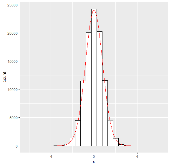
This pdf was the simplest form I could make.(maybe due to lack of my ability) I simulated this function and it looks fine.

The histogram is the simulated distribution of x and the line is gotten from this pdf. I attached the source code I ran at the end of the post.

I tried to get closed form but I couldn't

I was inspired from here, so I differentiated it with respect to x and after some doing math, I got $$\frac{\partial f_X(x)}{\partial x}=-\frac{2\sqrt2}{\pi \sigma^2} e^{-s^2/2} \int^\infty_0 \frac{1}{z}e^{-z^2}sinh(sz)dz$$

I couldn't do this integration by myself so I put it wolframalphaand it turns out 'imaginary error function'. I don't know about it but I guess this means it would be hard to get closed form of this function. So maybe the pdf form I wrote above the graph would be the best, in my opinion.

I feel sorry that I post this as an answer while I couldn't figure out the closed form of this integration.

Any correction and proofread is completely welcome. Thank you for reading this.

#simulation 1
sigma<-1
n_sim=100000
theta1<-rnorm(n_sim,0,sigma)
theta2<-rnorm(n_sim,0,sigma)

x<-c()
for(i in 1:n_sim){
x[i]<-runif(1)*(max(theta1[i],theta2[i])-min(theta1[i],theta2[i]))+min(theta1[i],theta2[i])
}



#simulation2
fx<-function(x,sigma){
nsim=3000
z<-abs(rnorm(nsim)) # 2 phi(z)
s<-sqrt(2)*x/sigma

C<-c()
for(i in 1:nsim){
C[i]<-1/z[i]*(pnorm(s+z[i])-pnorm(s-z[i]))
}
return(mean(C)/sigma)
}

graph_x<-seq(-6,6,0.1)
graph_y<-c()
for(i in 1:length(graph_x)){
graph_y[i]<-fx(graph_x[i],sigma)
}


#plotting simulation datas
library(ggplot2)

df1<-data.frame(x=x)
df2<-data.frame(x=graph_x, y=graph_y)
ggplot() +geom_histogram(data=df1, aes(x=x),binwidth=.5, colour="black", fill="white") #plot simul. 1
ggplot() +geom_line(data=df2, aes(x=x,y=y),color='red') #plot simul. 2

scale_factor=24000/0.7 # ratio of approximate maximum values between the histogram and the line graph
df2<-data.frame(x=graph_x, y=graph_y*scale_factor)

#this shows combined graph.
ggplot() +geom_histogram(data=df1, aes(x=x),binwidth=.5, colour="black", fill="white")+geom_line(data=df2, aes(x=x,y=y),color='red')