Bayesian p-value in wrong direction using step function in JAGS / BUGS

Question

I have estimated a Weibull regression model in JAGS using rjags and R2JAGS.

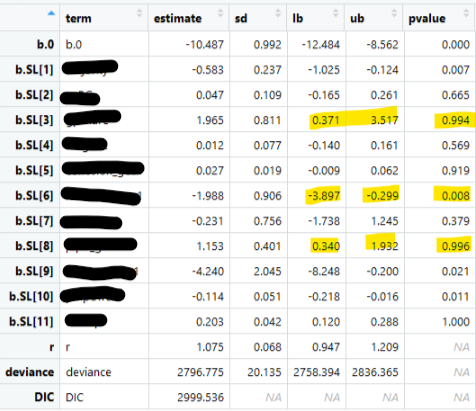
The estimated posterior predictive p-values using the step() function confuse me. They make sense (comparing them to lower and upper bound) when the estimated regression coefficients are negative but seem wrong, and almost like 1-p would be correct, when reg coefficients are estimated to be positive.

Is that just how the step function works? The thing is, in examples, I only see step functions implemented like: ppp.b.0 <- step(b.0) and never like ppp.b.0 <- 1-step(b.0) if b.0>0.

This is the result:

And this is the model:

modelstring.sl <- function() {
    for (i in 1:n.G) {  
        censored[i] ~ dinterval(t[i], t.cen[i])                         
        t[i] ~ dweib(r, mu[i]) # survival time ~ dweib(shape = r, scale = mu[i]) 
        log(mu[i]) <- b.0 + inprod(X.SL[i,], b.SL)  
    }

    # priors
    b.0 ~ dnorm(0.0, 0.0001) # intercept

    for (x in 1:n.XSL) {
        b.SL[x]  ~ dnorm(0.0, 0.0001) # reg coefs 
    }

    r ~ dexp(0.001) # shape parameter 

    var.G <- 1/(3.142^2/(6 *exp(2*log(r)))) # variance

    # ppp-values 
    for (x in 1:n.XSL) {             
        ppp.b.SL[x] <- step(b.SL[x])
    }
    ppp.b.0 <- step(b.0) 
}

# Data: character vector of variable names #
jags.data   <- c("t", "t.cen", "censored", "n.G", "X.SL", "n.XSL")

# Parameters: character vector of parameters to be monitored #
jags.params <- c("r", "var.G", "b.0", "b.SL", "ppp.b.SL", "ppp.b.0")

# Initial values in list form #
t.0 <- t
t.0[censored==0] <- NA
t.0[censored==1] <- t.cen[censored==1] + 5

jags.inits <- list( 
    list(t=t.0, b.0=0.0, b.SL=rep( 0.1,n.XSL), r=1.1), 
    list(t=t.0, b.0=0.1, b.SL=rep(-0.1,n.XSL), r=1.2), 
    list(t=t.0, b.0=0.2, b.SL=rep( 0.0,n.XSL), r=1.3))

# Run model with R2JAGS
 jagsfit.sl3 <- jags(data=jags.data, inits = jags.inits, parameters.to.save = jags.params, n.chains = 3, n.iter = iter, n.burnin = burnin, model.file = modelstring.sl)

Answer 1

The so-called 'Bayesian p-value' does not have the same interpretation as a true p-value: remember that you do not have a formal hypothesis test so there is no real concept of a 'probability of the data under the null hypothesis'. Instead, the probability that you are monitoring is simply the probability that the coefficient is greater than zero - which is arguably easier to interpret (and more useful) than a p-value ... but that's an entirely unrelated rant.

The answer is that your intuition is correct - you can simply take 1 minus the probability that the coefficient is positive to obtain the probability that the coefficient is negative, from which you could conclude (if this was probability was sufficiently small) that the coefficient most likely has a positive value. There is nothing wrong with this nor any particular reason why you could/should not (equivalently) monitor 1 minus the step function in the model.

But - here comes a more relevant rant - why are you focussed on imitating a p-value at all? It makes much more sense to look at the 95% credible intervals for the coefficient posterior directly, from which you can ascertain (1) if the 95% confidence interval does not include zero (i.e. the true value is likely either positive or negative - i.e. there is a true effect) but also importantly (2) the magnitude of the effect i.e. is it very likely to be a small (and potentially meaningless) effect or is it potentially a large (and therefore important) effect. Imitating a p-value loses this valuable information.