1
$\begingroup$

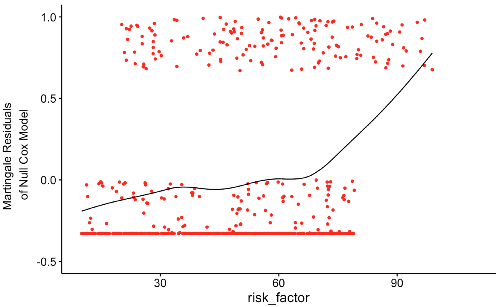
I have the following survival data: cases with a continuous variable risk_factor wich higher values having a higher HR (1.026, CI: [1.017-1.034], p = 2.03e-09) for survival (after running regression Cox model). I want to verify the log-linearity of the continuous variable risk_factor for predicting the survival. How could I do it? What would be the explanation and the code. Does it make sense to do it? Can it reinforce the information given by the Cox regression model?

library(broom)
library(tidyr)
timespan_censored = c(round(runif(450, 0, 4500), digit = 0), 
                  round(runif(150, 0, 1200), digit = 0))

risk_factor = c(runif(450, min=10, max=80), 
            runif(150, min=20, max=100))
status = c(rep(0, 450), rep(1, 150))
timespan_censored = c(round(runif(450, 0, 4500), digit = 0), 
                  round(runif(150, 0, 1200), digit = 0))
df_try = data.frame(status, timespan_censored, risk_factor)
cox_mod = coxph(Surv(timespan_censored, status) ~ risk_factor, data = df_try) %>% summary()
cox_mod

this is the output:

Call:
coxph(formula = Surv(timespan_censored, status) ~ risk_factor, 
data = df_try)

n= 600, number of events= 150 

                coef exp(coef) se(coef)     z Pr(>|z|)    
risk_factor 0.025294  1.025617 0.004219 5.995 2.03e-09 ***
---
Signif. codes:  0 '***' 0.001 '**' 0.01 '*' 0.05 '.' 0.1 ' ' 1

            exp(coef) exp(-coef) lower .95 upper .95
risk_factor     1.026      0.975     1.017     1.034

Concordance= 0.629  (se = 0.024 )
Rsquare= 0.062   (max possible= 0.953 )
Likelihood ratio test= 38.28  on 1 df,   p=6.133e-10
Wald test            = 35.94  on 1 df,   p=2.032e-09
Score (logrank) test = 37.31  on 1 df,   p=1.007e-09

ggcoxfunctional(Surv(timespan_censored, status) ~ risk_factor, data = df_try, xlim = c(10,110), ylim = c(-0.5,1.0))

output of of risk factor not transformed

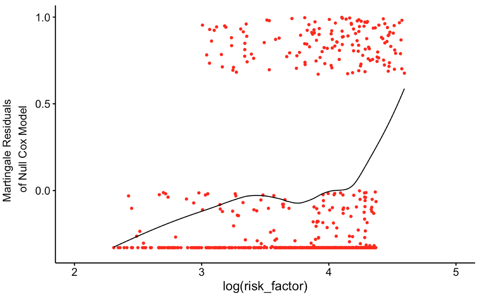
ggcoxfunctional(Surv(timespan_censored, status) ~ log(risk_factor), data = df_try, xlim = c(2,5), ylim = c(-0.35,1.0))

output of of risk factor log transformed

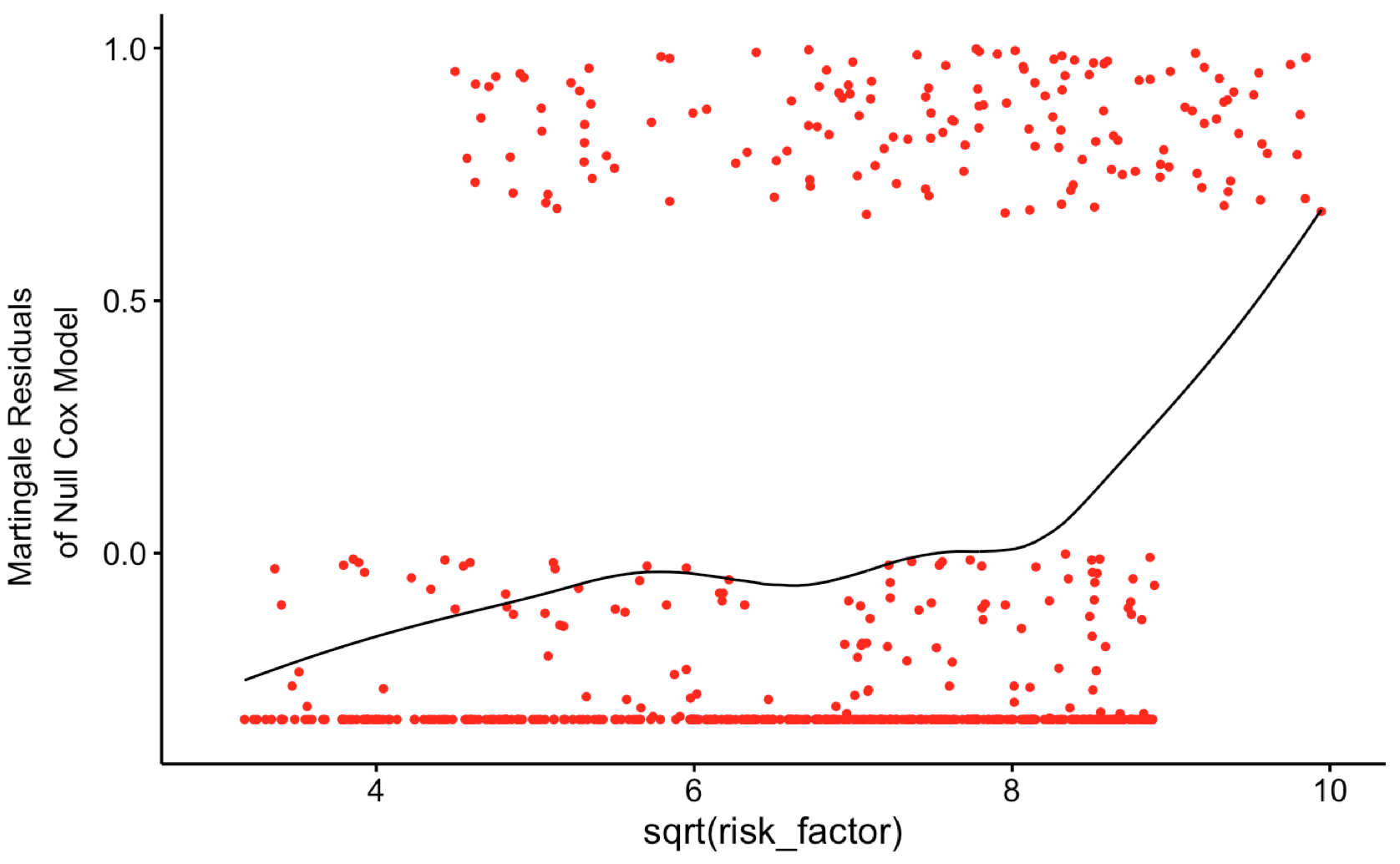
ggcoxfunctional(Surv(timespan_censored, status) ~ sqrt(risk_factor), data = df_try, xlim = c(3,10), ylim = c(-0.35,1.0))

output of of sqrt of risk factor

library(rms)
cox_mod_spline = coxph(Surv(timespan_censored,status)~ rcs(risk_factor,6))
cox_mod_spline
res = residuals(cox_mod_spline, type = "martingale")
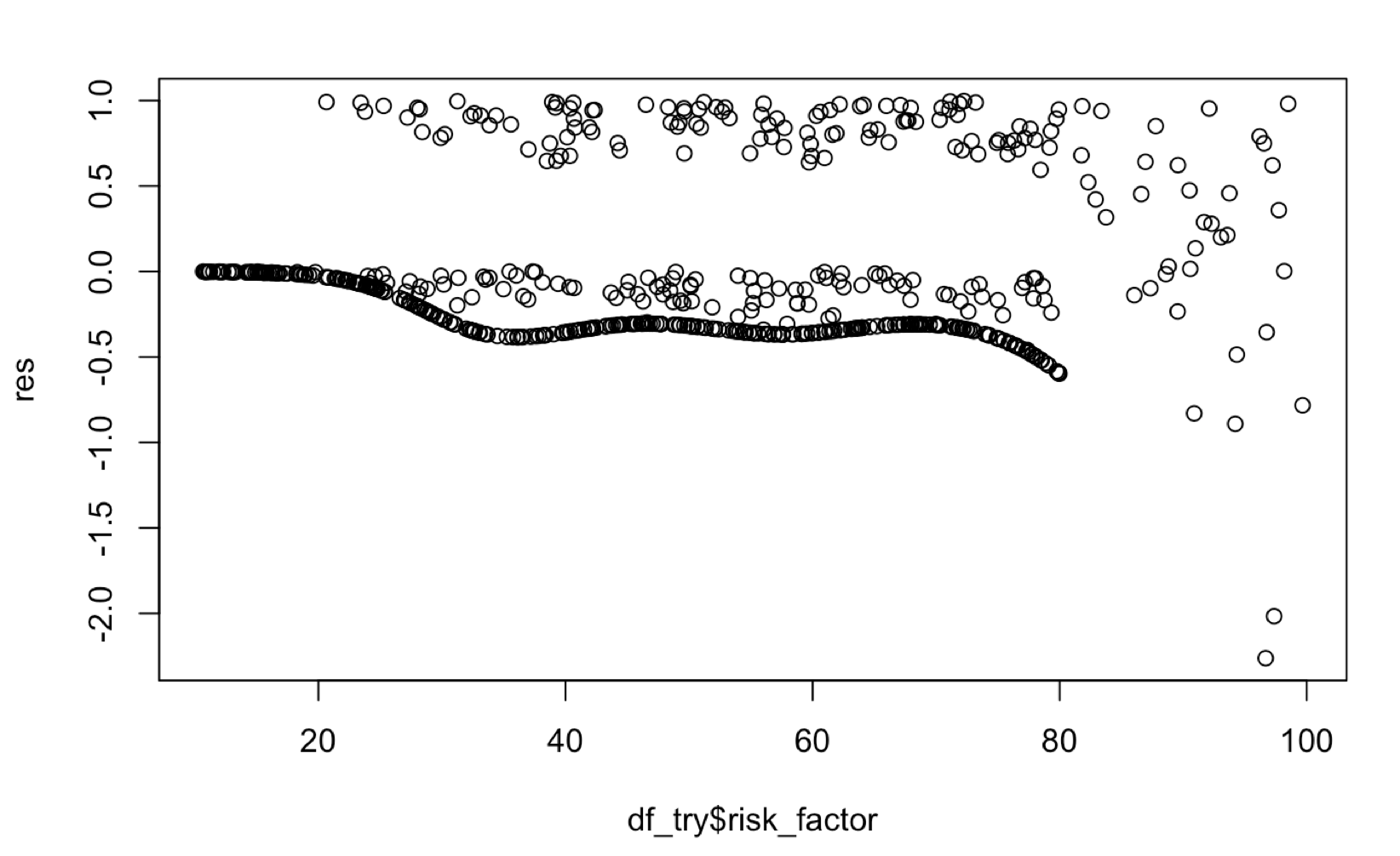
plot(df_try$risk_factor, res)

plot of the residuals of cox regression with 6 splines against risk factor

cox_mod_spline = coxph(Surv(timespan_censored,status)~ rcs(risk_factor,4))
cox_mod_spline
res = residuals(cox_mod_spline, type = "martingale")
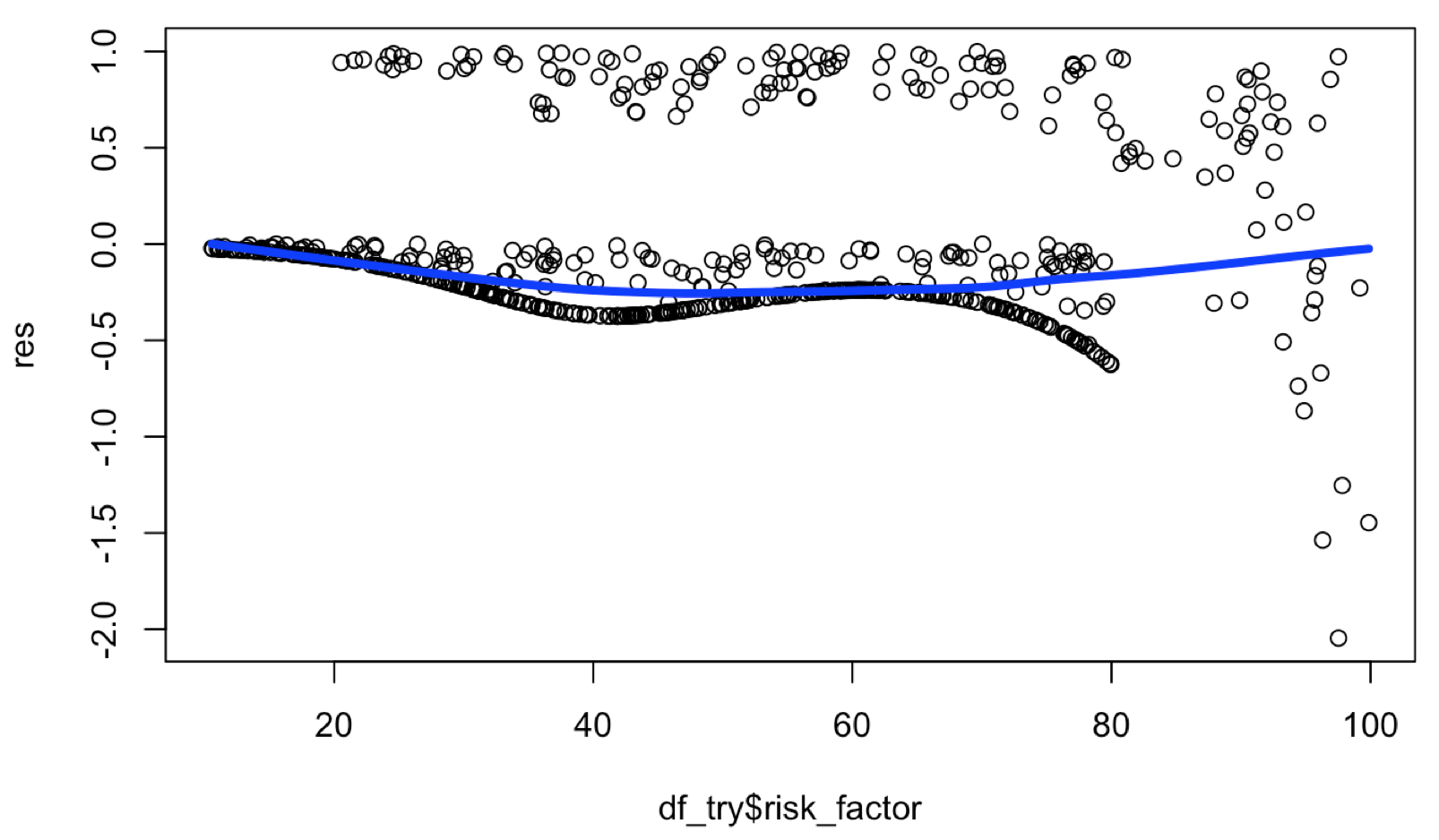
plot(df_try$risk_factor, res)
lines(loess.smooth(df_try$risk_factor, res), lwd = 4, col="blue")

loess line added to previous graph

$\endgroup$
9
  • $\begingroup$ The answer might depend on correlations with other predictors and numbers of events. Please read this answer, which includes information about using martingale residuals or splines of the continuous predictor to evaluate linearity; also this page for related discussion and some useful links. If you still have unanswered questions on evaluating linearity with respect to your log-transformed continuous predictor, please edit this question to provide the further details that you need clarified. $\endgroup$
    – EdM
    Commented Oct 5, 2018 at 15:12
  • $\begingroup$ The default choice of axis limits in ggcoxfunctional is not very good, as you might infer from discussion on the pages I linked to above. Specify the limits yourself (with xlim and ylim arguments) so that the y axis covers a range between -2 and +1 and so the x axis covers the complete range of your data, and post the new graphs instead, for a more complete look at what you have. $\endgroup$
    – EdM
    Commented Oct 5, 2018 at 17:23
  • $\begingroup$ Thank you very much for the very helpful comment @Edm. I'm trying to read all the details in the link you provided. It seems that the rms package is a package to be used when dealing with survival although I have to say that the survivaland survminerpackages are more beginner friendly. As I did a univariate cox regression, obtaining the Martingale residuals could be a good option. I performed the 2 transformations of variables. So I guess that now I have to choose the transformation that looks the most like a straight line. But none of the plots seem to do the job well $\endgroup$
    – ecjb
    Commented Oct 5, 2018 at 17:23
  • $\begingroup$ Thanks (again!) for the good tip @Edm. I changed the axes of the graphs and updated the pictures. I still don't see a model which is definitely better than the other ones. $\endgroup$
    – ecjb
    Commented Oct 5, 2018 at 17:36
  • $\begingroup$ Try a restricted cubic spline transformation of your risk_factor. Without fully learning the rms package you can still load it to get its rcs() function for a standard coxph() call, for example: coxph(Surv(time,status)~ rcs(risk_factor,3), for a spline with 3 knots (you might want/need to use more). Plot martingale residuals from the coxph object with the spline transformation against risk_factor; a reasonably flat line shows you handled non-linearity with the spline. You'll have to plot that yourself as ggcoxfunctional() only shows residuals from the null model. $\endgroup$
    – EdM
    Commented Oct 5, 2018 at 17:58

1 Answer 1

3
$\begingroup$

You can fit a Cox model that relaxes the linearity assumption for the risk_factor on the log hazard scale, using, e.g., splines. You could compare this model with the linear fit using a likelihood ratio test and see if the effect is linear or not. If it is nonlinear, you can depict it with an effects plot.

The code below illustrates these steps with your simulated data:

library("survival")
library("lattice")
library("splines")

# simulate the data
timespan_censored <- c(round(runif(450, 0, 4500), digit = 0), 
                       round(runif(150, 0, 1200), digit = 0))
risk_factor <- c(runif(450, min = 10, max = 80), 
                 runif(150, min = 20, max = 100))
status <- c(rep(0, 450), rep(1, 150))
timespan_censored <- c(round(runif(450, 0, 4500), digit = 0), 
                       round(runif(150, 0, 1200), digit = 0))
df_try <- data.frame(status, timespan_censored, risk_factor)

# fit a Cox model with a linear effect for 'risk_factor'
cox_mod1 <- coxph(Surv(timespan_censored, status) ~ risk_factor, data = df_try)

# fit a Cox model with a nonlinear effect for 'risk_factor' using natural cubic splines
cox_mod2 <- coxph(Surv(timespan_censored, status) ~ ns(risk_factor, 4), data = df_try)

# likelihood ratio test for linearity
anova(cox_mod1, cox_mod2)

# Create an effect plot to depict the relationship
ND <- with(df_try, data.frame(risk_factor = seq(min(risk_factor), 
                                                max(risk_factor), length.out = 500)))

prs <- predict(cox_mod2, newdata = ND, type = "lp", se.fit = TRUE)
ND$pred <- prs[[1]]
ND$se <- prs[[2]]
ND$lo <- ND$pred - 1.96 * ND$se
ND$up <- ND$pred + 1.96 * ND$se

xyplot(pred + lo + up ~ risk_factor, data = ND,
       type = "l", col = "black", lwd = 2, lty = c(1, 2, 2),
       abline = list(h = 0, lty = 2, lwd = 2, col = "red"),
       xlab = "Risk Factor", ylab = "log Hazard Ratio")

You can find more examples in my Survival Analysis in R Companion for my survival course.

$\endgroup$
1
  • $\begingroup$ Thank you very much for your very good answer @DimitrisRizopoulos. I'm definitely going to have a look to your course and your blog and make the practical cases. However, I have some questions: 1. Although it fits the log hazard ratio is 0 for the intermediate value, it is a bit far off in the extreme value. No? 2. What should be the best interpretation of the analysis? "using cubic splines with 4 knots, the variable risk factor reasonably approached a constant 0 value of the log hazard ratio"? $\endgroup$
    – ecjb
    Commented Oct 5, 2018 at 20:47

Your Answer

By clicking “Post Your Answer”, you agree to our terms of service and acknowledge you have read our privacy policy.

Not the answer you're looking for? Browse other questions tagged or ask your own question.