Why does increasing the sample size of coin flips not improve the normal curve approximation?

Question

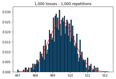
I'm reading the Statistics (Freeman, Pisani, Purves) book and I'm trying to reproduce an example where a coin is tossed say 50 times, the number of heads counted and this is repeated say 1,000 times.

1. First, I kept the number of tosses (sample size) at 1000 and increased the repetitions. The more repetitions, the better the data fit the normal curve.

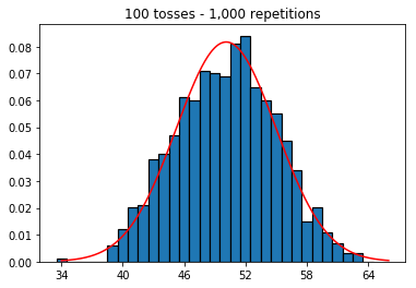
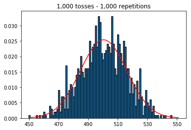
2. So next, I tried keeping the number of repetitions fixed at 1,000 and increased the sample size. The larger the sample size, the worst the normal curved seemed to fit the data. This seems to be contradictory to the book example which better approximates the normal curve as the sample size increases.

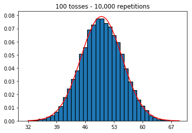
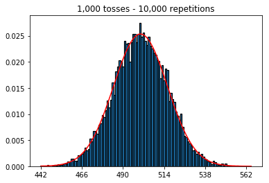
3. I wanted to see what would happen if I increased the sample size, but with a larger number of repetitions which were fixed at 10,000. This seems to also contradict the book.

Any ideas what I'm doing wrong?

Code and graphs below.

%matplotlib inline

def plot_hist(num_repetitions, num_tosses):
    tosses = np.random.randint(0, 2, size=[num_repetitions, num_tosses])
    sums = np.apply_along_axis(lambda a: np.sum(a == 1), 1, tosses)

    xmin, xmax = min(sums), max(sums)  
    lnspc = np.linspace(xmin, xmax, len(sums))

    m, s = stats.norm.fit(sums) # get mean and standard deviation  
    pdf_g = stats.norm.pdf(lnspc, m, s) # now get theoretical values in our interval  

    bins = np.arange(xmin, xmax) - 0.5
    step = int((xmax - xmin)/5)

    fig, ax = plt.subplots()
    _ = ax.hist(sums, bins, edgecolor='black', linewidth=1.2, density=True)
    _ = ax.plot(lnspc, pdf_g, label="Norm", color='red')
    _ = ax.set_xticks(bins[::step] + 0.5)
    _ = ax.set_title('{:,} tosses - {:,} repetitions'.format(num_tosses, num_repetitions))

1. Experiment with increasing number of repetitions (fixed sample size of 1000)

plot_hist(1000, 1000)

plot_hist(10000, 1000)

plot_hist(100000, 1000)

2. Experiment with increasing sample size (fixed at 1000 repetitions)

plot_hist(1000, 100)

plot_hist(1000, 1000)

plot_hist(1000, 10000)

3. Experiment with increasing sample size (fixed at 10,000 repetitions)

plot_hist(10000, 100)

plot_hist(10000, 1000)

plot_hist(10000, 10000)

plot_hist(10000, 100000)

Answer 1

In the second case, by increasing the number of tosses, you increase the number of bins a single trial can fall into. While the first case of experiment 2 only has a maximum of 100 bins that can be filled, the last example has 10000 bins. You increased the "resolution" of your experiment by a factor 100 (i.e., one bin in your first experiment is now represented by roughly 100 in your second). Of course this means that you would expect to require a factor 100 more data to fill your bins.

Answer 2

You can think of an individual coin flip as an independent Bernoulli trial. One trial will give you either heads/tails or success/failure, respectively. If you repeat this say 100,000 times, the average number of heads will be very close to 0.5, if the coin is fair.

Now if you increase the number of trials to 1,000 and keep the repetition at 1, you will get a sequence of 1,000 successes/failures and cannot say much about the probability of observing, on average, 500 heads unless you increase the number of repetitions for each of those independent trials. As the number of repetitions increases, you will get a better and better approximation to the normal distribution.

For me it is easier to think of the trials not as “tosses” or “sample sizes” but instead of separate coins and the repetitions as the number of flips of each of those coins. Then it also makes intuitively sense that by increasing the number of coins (or trials), while keeping the total number of repetitions (or flips) constant, the approximation of the data to the normal distribution gets worse.

Answer 3

I think the other answers here are great, but wanted to add an answer that extends to another statistical tool.

You're starting with a baseline that you think should approximate a normal curve, and then going from there to see if you can better approximate a normal curve. Try going the other direction, and see what you can do to do a worse job at approximating. Try simulations where you have 10 flips and 1000 repetitions. Compare this to simulations where you have 1000 flips and 10 repetitions. It should be clear that the former case has the better approximation.

The extension that I want to make is to ANOVA (analysis of variance). You see a lot of new data scientists that have a poor grasp of this problem, and design their studies so that they have a lot of flips, but few repetitions. They have a lot of data, but it says less than they'd like. Like measuring every leaf on a tree, but only having two trees. We can say quite a bit about leafs on those two trees, but not leafs on trees in general. You'd have been better off getting a much smaller sample of leafs, and getting a lot of trees.

Answer 4

To gain some additional intuition consider the following:

Imagine you do only one single repetition.

In that case you can increase the number of tosses all you want but it is not gonna resemble a normal distribution. And this makes sense since your histogram is only gonna have one single peak.

---

The normal distribution is an approximation for the probabilty distribution (of the binomial distribution).

What you did was not creating this distribution. But instead , you approximated this distribution by using a limited (and small) number of simulations. (and what you discovered is that this approximation becomes worse when you increase the number of bins in the histogram)

---

So you both need a high number of tosses and repetitions.

• when the number of tosses is high then the binomial distribution (multiple coin tosses) can be approximated by normal distribution.
• when the number of repetitions/simulations is high than histogram of these experiments approximates the density of the binomial distribution.