What's the right test of significance for a categorical independent variable and categorical dependent variable?

Question

I have data that looks like this. It goes on for about 10,000 rows. Goal is always TRUE/FALSE and category has five options.

   category      goal
1 TWO LEGS     FALSE
2 TWO LEGS     TRUE
3 FOUR LEGS    TRUE
4 FOUR LEGS    FALSE
5 ONE LEG      FALSE
6 TWO LEGS     FALSE
  ...          ...

I'd like to be able to tell if one of the categories is True more frequently than the other categories in a way that is statistically significant. I'd like to test the null hypothesis that each category has the same proportion of true cases as all the other categories.

What's the right test for that?

Answer 1

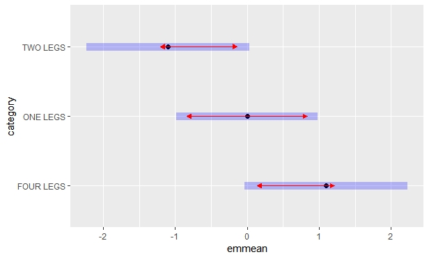
You can use emmeans package coupled with a logistic model to determine if there is a statistical difference between any category and specific categories. The emmeans package performs tukey pairwise comparisons of estimated marginal means (ls means) by default, i.e., statistically tests which categories are different from each other. Additonally, logistic models are used for modeling and assessing binary outcomes like TRUE or FALSE and 1 or 0.

Below I have built a sample data set similar to yours, run a logistic model, and have run a post-hoc (emmeans tukey comparison) to assess statistical differences in categories. You can use this as a start framework. Keep in mind your results may differ from mine as my data are not exactly the same as yours.

Code:

#### Making mock data set similar to yours########
data = as.data.frame(list(c("TRUE", "FALSE","FALSE","FALSE",
                        "TRUE","TRUE","TRUE","FALSE",
                        "FALSE","FALSE","TRUE","TRUE"),
                      c("TWO LEGS","TWO LEGS","TWO LEGS","TWO LEGS",
                        "FOUR LEGS","FOUR LEGS","FOUR LEGS","FOUR LEGS",
                        "ONE LEGS","ONE LEGS","ONE LEGS","ONE LEGS")))

colnames(data) = c("goal", "category")
data = rbind(data,data,data,data)

#### Import required packages ####
library(emmeans)


#### Build model and do some hypothesis testing ###
model = glm(goal ~ category, data=data, family = binomial(link = "logit"))
summary(model)# general model evaluation, are any of the categories (coefficients) significant


#### Post-hoc test to determine statistical difference between category levels ###

marg_means = emmeans(model, "category") #estimate mariginal means by category
contrast(marg_means, method="pairwise", adjust = "tukey" )
plot(marg_means , comparisons =TRUE)# Pairwise comaparisons plot, visual representation
cld(marg_means) #grouping numbers illustrate which categories are different from each other

Below I have provided the output from my example and a basic explanation.

Output:

Results of summary statement: Because your using a factor variable (category) the model will estimate a separate coefficient (regressor) for each different level (i.e., category). While you can easily see to the coefficient for one leg and two legs, the coefficient for four legs is simply the intercept. I am going to skip over explanation of how to use these to make a prediction, as you are interested in hypothesis testing and it will lead us down the rabbit hole. The next step is to run post-hoc tests via emmeans to determine which category levels are different. As is the case in my example.

Call:
glm(formula = goal ~ category, family = binomial(link = "logit"), 
data = data)

Deviance Residuals: 
Min       1Q   Median       3Q      Max  
-1.6651  -0.8632   0.0000   0.8632   1.6651  

Coefficients:
             Estimate Std. Error z value Pr(>|z|)   
(Intercept)        1.0986     0.5773   1.903  0.05706 . 
categoryONE LEGS  -1.0986     0.7638  -1.438  0.15031   
categoryTWO LEGS  -2.1972     0.8165  -2.691  0.00712 **
---
Signif. codes:  0 ‘***’ 0.001 ‘**’ 0.01 ‘*’ 0.05 ‘.’ 0.1 ‘ ’ 1

(Dispersion parameter for binomial family taken to be 1)

Null deviance: 66.542  on 47  degrees of freedom
Residual deviance: 58.170  on 45  degrees of freedom
AIC: 64.17

Number of Fisher Scoring iterations: 4

Results of the contrast statement: If you look at the p-values you can see that four legs category is statistically different from two legs ($\alpha$ = 0.05), but there are no other statistical differences between any of the other categories. You can look at the estimate for the statistical comparisons that were significant to understand the directionality of the difference. What do I mean by this, for the FOUR LEGS - TWO LEGS comparison the estimate is positive (2.2) this implies that four legs are more likely to be TRUE (i.e., have a goal value of TRUE) than two legs. However, if the estimate was negative it would imply the opposite.

contrast             estimate    SE  df z.ratio p.value
FOUR LEGS - ONE LEGS      1.1 0.764 Inf 1.438   0.3211 
FOUR LEGS - TWO LEGS      2.2 0.816 Inf 2.691   0.0195 
ONE LEGS - TWO LEGS       1.1 0.764 Inf 1.438   0.3211 

Results of the plot statement: This is just a visual representation of the emmeans comparisons. See the additional reading link below for more detail.

Results of the cld statement: This is another visual representation of the comparisons. The different grouping numbers ( 1,2) indicate which categories are different. Two legs (group 1) is different than four legs ( group 2), but not one legs ( group 1 and group2).

category  emmean    SE  df asymp.LCL asymp.UCL .group
 TWO LEGS    -1.1 0.577 Inf    -2.230     0.033  1    
 ONE LEGS     0.0 0.500 Inf    -0.980     0.980  12   
 FOUR LEGS    1.1 0.577 Inf    -0.033     2.230   2   

Here are some links for additional online resources and reading

These links explains the basics and use of glm used for the logistic model https://www.rdocumentation.org/packages/stats/versions/3.5.2/topics/glm

https://www.r-bloggers.com/what-does-a-generalized-linear-model-do/

This link explains the basics of emmeans (estimated marginal means ):

https://cran.r-project.org/web/packages/emmeans/vignettes/basics.html

This link explains the emmeans package:

https://www.rdocumentation.org/packages/emmeans

This link explains contrasts (post-hoc comparisons ) via emmeans package:

https://cran.r-project.org/web/packages/emmeans/vignettes/comparisons.html

For additional reading on linear models and there extensions (glm, glmm, etc.) I recommend the following book

https://www.crcpress.com/Extending-the-Linear-Model-with-R-Generalized-Linear-Mixed-Effects-and/Faraway/p/book/9781498720960

Answer 2

If you are looking for a simple test and not for a model like in Devon's answer, and if there is no order in your category variable, I think you just want to perfom a simple khi-square test.

In R, it will look like this:

chisq.test(df$category, df$goal) #assuming your dataframe is named "df"

Please note that this will test the exact null hypothesis you mentioned, but if you want to analyse the difference between some categories only, you will have to do post-hoc analysis, which is not always a good thing.

If your category is ordered though (if you have 2 legs < 4 legs < 6 legs etc), you should then code your variable as ordered and use the Cochran-Armitage test for trend.