9
$\begingroup$

Why does larger perplexity tend to produce clearer clusters in t-SNE?

By reading the original paper, I learned that the perplexity in t-SNE is $2$ to the power of Shannon entropy of the conditional distribution induced by a data point. And it is mentioned in the paper that it can be interpreted as a smooth measure of the effective number of neighbors.

If the conditional distribution of a data point is constructed by Gaussian distribution (SNE), then the larger the variance $\sigma^2$, the larger the Shannon entropy, and thus the larger the perplexity.

So, the intuition that I built is:

The larger the perplexity, the more non-local information will be retained in the dimensionality reduction result.

When I use t-SNE on two of mine test datasets for dimensionality reduction, I observe that the clusters found by t-SNE will become consistently more well-defined with the increase of perplexity. Although this is a desirable outcome, I just cannot explain this with the intuition that I just built.

Here is the result that I have, the data and the script used for generating the figure have been uploaded here: result

Besides the confusion that I just mentioned, I also don't know how to interpret the result.

What could be a possible explanation for the fact that it is easier for t-SNE to find well-defined clusters in Random dataset then Benchmark dataset?

$\endgroup$
13
  • $\begingroup$ Interesting labels. What data are that? What's the difference between the two data sets? "Random" data set is not truly random, is it? $\endgroup$
    – amoeba
    Commented Mar 28, 2019 at 8:20
  • 1
    $\begingroup$ @amoeba The data are atomic fingerprints for describing local atomic environments. As you can see from the labels of the clusters, there are 50 atoms (Li, Ge, P, and S) in the system I'm studying. By taking into account the symmetry, there should be 9 clusters. Because I'm using a batch of different atomic configurations for dimensionality reduction, the name 'Benchmark' refers to a batch which has some nice property, and 'Random' refers to a batch of configurations that are just randomly sampled from a large batch of configurations. $\endgroup$ Commented Mar 28, 2019 at 8:31
  • $\begingroup$ Thanks. The Benchmark dataset has really curious structure visible with very low perplexity: looks like it consists of 1-dimensional segments. Does it make sense to you? $\endgroup$
    – amoeba
    Commented Mar 28, 2019 at 11:17
  • $\begingroup$ @amoeba Thank you! I was thinking whether the 1-dimensional segments make sense. Because the structures in the benchmark dataset are not so different from each other (which is unlike the random dataset where structures are just randomly sampled from a really large dataset), it might be reasonable that there are many 1-dimensional segments of consistent colors. However, I don't know whether the segments can be interpreted as clusters, and I also learned t-SNE does not preserve distances and cluster size, so I really can't say whether it makes sense to me... $\endgroup$ Commented Mar 30, 2019 at 1:50
  • 1
    $\begingroup$ @amoeba Thank you! After looking deeper into the process of how the benchmark dataset is generated, I think I understand why there are so many one-dimensional segments, the atomic fingerprints are heavily correlated! I wrote a toy example to demonstrate the process of how the structures are sampled, the result of this toy example is almost the same as the one I posted. $\endgroup$ Commented Apr 3, 2019 at 12:45

2 Answers 2

12
$\begingroup$

The larger the perplexity, the more non-local information will be retained in the dimensionality reduction result.

Yes, I believe that this is a correct intuition. The way I think about perplexity parameter in t-SNE is that it sets the effective number of neighbours that each point is attracted to. In t-SNE optimisation, all pairs of points are repulsed from each other, but only a small number of pairs feel attractive forces.

So if your perplexity is very small, then there will be fewer pairs that feel any attraction and the resulting embedding will tend to be "fluffy": repulsive forces will dominate and will inflate the whole embedding to a bubble-like round shape.

On the other hand, if your perplexity is large, clusters will tend to shrink into denser structures.

This is a very handway explanation and I must say that I have never seen a good mathematical analysis of this phenomenon (I suspect such an analysis would be nontrivial), but I think it's roughly correct.


It is instructive to see it in a simulation. Here I generated a dataset with six 10-dimensional Gaussian balls ($n=1000$ in each ball) that are located very far away from each other --- so far that even for perplexity 100 all attractive forces are within-cluster. So for perplexities between 5 and 100, shown below, there are never any attractive forces between clusters. However, one can clearly see that the clusters "shrink" when perplexity grows.
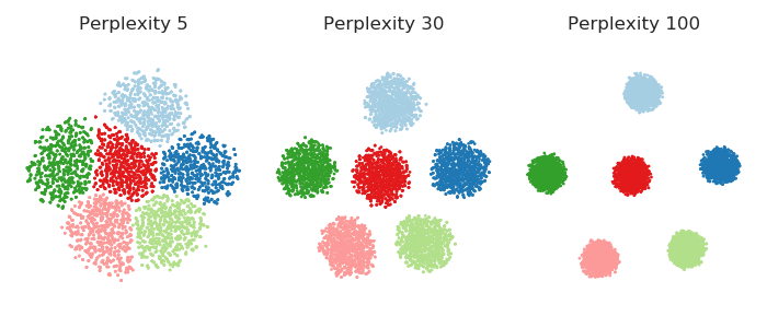
enter image description here

In fact, one can get rid of perplexity entirely, and make each point feel equally strong attraction to its closest $K$ neighbours. This means that I replace the Gaussian kernel in the high-dimensional space with the "uniform" kernel over the closest $K$ neighbours. This should simplify any mathematical analysis and is arguably more intuitive. People are often surprised to see that the result very often looks very similar to the real t-SNE. Here it is for various values of $K$:
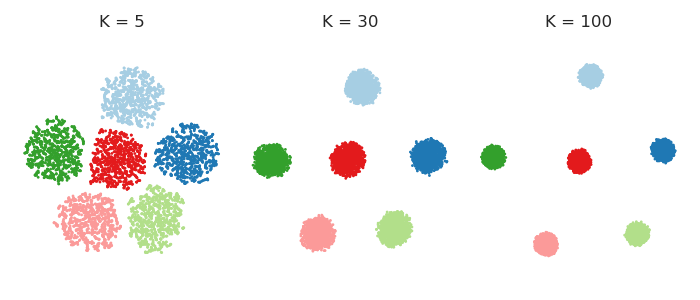
enter image description here


Code

%matplotlib notebook

import numpy as np
import pylab as plt
import seaborn as sns

sns.set_style('ticks')

# https://github.com/KlugerLab/FIt-SNE
import sys; sys.path.append('/home/localadmin/github/FIt-SNE')
from fast_tsne import fast_tsne

col = np.array(['#a6cee3','#1f78b4','#b2df8a','#33a02c','#fb9a99',
                '#e31a1c','#fdbf6f','#ff7f00','#cab2d6','#6a3d9a'])

n = 1000  # sample size per class
p = 10    # dimensionality
k = 6     # number of classes
d = 10    # distance between each class mean and 0

np.random.seed(42)
X = np.random.randn(k*n, p)
for i in range(k):
    X[i*n:(i+1)*n, i] += d

perpl = [5, 30, 100]
Z1 = []
for p in perpl:
    Z = fast_tsne(X, perplexity=p, seed=42)
    Z1.append(Z)

ks = [5, 30, 100]
Z2 = []
for kk in ks:
    Z = fast_tsne(X, K=kk, sigma=10000, seed=42)
    Z2.append(Z)


fig = plt.figure(figsize=(7, 3))

for i,Z in enumerate(Z1):
    plt.subplot(1,3,i+1)
    plt.axis('equal', adjustable='box')
    plt.scatter(Z[:,0], Z[:,1], s=1, c=col[np.floor(np.arange(n*k)/n).astype(int)])
    plt.title('Perplexity {}'.format(perpl[i]))
    plt.gca().get_xaxis().set_visible(False)
    plt.gca().get_yaxis().set_visible(False)

sns.despine(left=True, bottom=True)
plt.tight_layout()
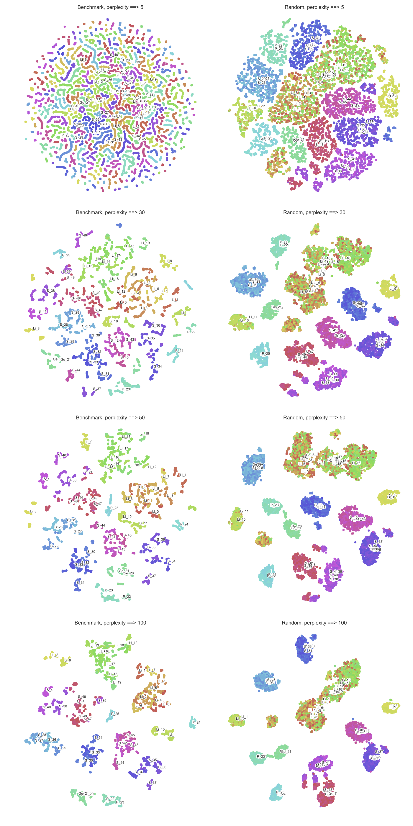

fig = plt.figure(figsize=(7, 3))

for i,Z in enumerate(Z2):
    plt.subplot(1,3,i+1)
    plt.axis('equal', adjustable='box')
    plt.scatter(Z[:,0], Z[:,1], s=1, c=col[np.floor(np.arange(n*k)/n).astype(int)])
    plt.title('K = {}'.format(perpl[i]))
    plt.gca().get_xaxis().set_visible(False)
    plt.gca().get_yaxis().set_visible(False)

sns.despine(left=True, bottom=True)
plt.tight_layout()
$\endgroup$
3
$\begingroup$

I believe this is because of this mismatch in t-SNE between the input (Gaussian) and output (student-t) distributions. It is beneficial to make such blobs in order to separate from everything else as required by the long tail of the t-distribution. The repulsive forces dominate.

In such cases SNE may work better. Have you tried?

$\endgroup$
5
  • $\begingroup$ I will try SNE, but I can't find a piece of python code that implements SNE... $\endgroup$ Commented Apr 2, 2019 at 7:19
  • $\begingroup$ @meTchaikovsky You can do SNE with the code posted above in my answer and adding df=100 (or other large number) to the fast_tsne call. See here arxiv.org/abs/1902.05804. I am not aware of any other implementation of SNE suitable for large datasets. By the way, I tried adding df=100 to the code posted above (with toy examples); I expected to see qualitatively the same thing, but Anony-Mousse's intuition seems to have been right: perplexities 5, 30, and 100 produced very similar embedding and I couldn't get a bubble-like "inflation" with small perplexities. $\endgroup$
    – amoeba
    Commented Apr 2, 2019 at 9:44
  • $\begingroup$ Blame Gboard autocorrect... $\endgroup$ Commented Apr 2, 2019 at 17:20
  • $\begingroup$ Thanks for the edit. But how do you explain the difference between small and large perplexity? Look at my toy simulations. Not sure I understand how your answer explains that. $\endgroup$
    – amoeba
    Commented Apr 2, 2019 at 18:41
  • $\begingroup$ With larger perplexity the near neighbors become more evenly similar (and hence can be contracted more) but the mismatch with the long tail increases, and it pushes away all the far points even more. That is my guess. $\endgroup$ Commented Apr 2, 2019 at 21:59

Your Answer

By clicking “Post Your Answer”, you agree to our terms of service and acknowledge you have read our privacy policy.

Not the answer you're looking for? Browse other questions tagged or ask your own question.