Beginner : Interpreting Regression Model Summary [duplicate]

Question

> sal <- read.csv("/Users/YellowFellow/Desktop/Salaries.csv",header 

= TRUE)
> regressionModel = lm(sal$Salary~sal$Yrs.since.phd)
> summary(regressionModel)

Call:

lm(formula = sal$Salary ~ sal$Yrs.since.phd)

Residuals:
   Min     1Q Median     3Q    Max 
-84171 -19432  -2858  16086 102383 

Coefficients:
                  Estimate Std. Error t value Pr(>|t|)    
(Intercept)        91718.7     2765.8  33.162   <2e-16 ***
sal$Yrs.since.phd    985.3      107.4   9.177   <2e-16 ***
---
Signif. codes:  0 ‘***’ 0.001 ‘**’ 0.01 ‘*’ 0.05 ‘.’ 0.1 ‘ ’ 1

Residual standard error: 27530 on 395 degrees of freedom
Multiple R-squared:  0.1758,    Adjusted R-squared:  0.1737 
F-statistic: 84.23 on 1 and 395 DF,  p-value: < 2.2e-16

The above is my result from the basic linear model that I've created. I've been trying to interpret these results for some time but I don't understand the mathematical formula's behind them or how to explain results such as Coefficients, Residuals & Multiple R-squared. Please be kind enough to explain this to me in a simplified manner.

Answer 1

Let's make sure we are on the same page: you are estimating a model following the form $Y <- \beta_0 + \beta_1X + \epsilon$ where $\epsilon$ is a random variable that follows a normal distribution (zero-mean, and an unknown $\sigma$ standard deviation) Of course, $\beta_0, \beta_1$ and don't forget $\sigma$! is what we are trying to get by fitting the model to our data.

Let's focus first on the coefficients: the "estimates" are easy: they are just the estimated values for $\beta_0$ and $\beta_1$ ("intercept" and "Salary" respectively). They are not the real $\beta_0$ and $\beta_1$, but rather the most reasonable values given the data on the sample. You are also told the standard estimation error. The t-value is nothing but the ratio between estimation and standard estimation error. If it is big, you will get a small p-value (like that 2.2e-16, or 0.00000000000000002) The p-value the result of a test for the hypothesis "$\beta_1$ (or the corresponding parameter) is a actually 0". That low p-value is telling you that "nobody believes $\beta_1$ to be 0. And what $\beta_1 \neq 0$ means is that $X$ is relevant in predicing $Y$

Above the coefficients, you have information about the residuals. The residuals are nothing but the distance between your data and what your model predicts for the data (remember, we have just a straight line, so most points of the training dataset will lay somewhere near it, but not exactly on it) Minimum and maximum are pretty self-explanatory. 1Q is the smaller value that is bigger than 25% of the residuals. Same about median (50%) and 3Q (75%) On the bottom of you have the standard error of the residuals (we don't talk about mean of residuals because it's always 0. Residuals are nothing but estimations of $\epsilon$) and its standard deviation is a good estimation for $\sigma$

The output also mentions degrees of freedom (for linear regression, number of observations - number of parameters) R-squared ($R^2$) measures goodness-of-fit (i.e.: what part of the variance in the target variable is explained by your model. In case of simple regression, it's just the square of the correlation coefficient between $Y$ and $X$) The adjusted $R^2$ is the same thing but compensating for the number of parameters (theoretically, we good increse our $R^2$ just by including more and more variables, without that meaning that the model is better. Adjusted $R^2$ is useful when comparing models with different number of parameters, so in simple regression we don't really care too much)

The final line is a test on whether every parameter $\beta$, non including $\beta_0$ is different from 0. As we only have $\beta_1$, it is equivalent to the test we have on the coefficients block for $\beta_1=0$

Answer 2

"formula's behind them or how to explain results such as Coefficients, Residuals & Multiple R-squared"

Formula: $\hat y = b_{0} + b_{1} * x_{i} $

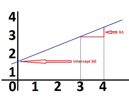
Coefficients: You have an intercept $b_{0}$ of 2.033 and regression weight $b_{1}$ of 1.784e-04.

To visualize what that means look the following plot:

The intercept is the value on the $y$ axis if $x= 0$ because $\hat y = b_{0} + b_{1} * 0 = \hat y = b_{0}$. Visually speaking that is the point where the regerssion line crosses the $y$ axis.

The $b_{1}$ coefficient tells you how the predicted $\hat y$ values cahnge if $x$ changes by +1. Hence, a positive $b_{1}$ coefficient indicates an increasing and a negative $b_{1}$ coefficient indicates a falling regression line. In your case this means that if the x value is zero the dependend variable y is 2.033. Further, if x increases by 1, the dependent variable y increases by 1.784e-04.

Residuals: You can make predictions with the formula above. You can predict what $y$ someone should have with a $x$ of 12,000, for example. In your case that would be:

$\hat y = 2.033 + 1.784e-04 * 12,000 = 4.1738$

So accordnign to your model someone with a $x$ of 12,000 should have a y of 4.1738. But it may be that there actually are people in your dataset with a $x$ of 12,000 and it is likely that their actual y value is not exactly 4.1738 but let's say 6.1738 and 2.1738. So your prediction made some mistake which is 6.1738 - 4.1738= 2 for one and 2.1738 - 4.1738= -2 for the other person. As you can see the predicted value can be too high or too low and this could give a mean error of 0 (like here: mean of +2 and -2 is 0). This would be misleading because an error of zero implies there is no error. To avoid that we usually use squared the error values, i.e. (6.1738 - 4.1738)$^{2}$ and (2.1738 - 4.1738)$^{2}$. By the way, in OLS the regression coefficients are estimated by "minimizing the sum of the squares of the differences between the observed dependent variable (values of the variable being predicted) in the given dataset and those predicted by the linear function" (see here).

R-square: This value tells you the proportion of the variation of your dependent variable y that was explained with the regression model. In your model the predictor explained 17.58% of the variation in your dependent variable. Keep in mind that you should use an adjusted version of R-squared if you want to compare models with different numbers of predictors.

Note that you write sal$Yrs.since.phd ~ sal$Salaryand if Yrs.since.phd means "years since Phd" it should possibly be the other way around: what you maybe want to do is to predict the salary of a person with the years since the Phd and not to predict the years since Phd with the salary. If so, you can simply switch both variables.