Method: Simulation assuming multivariate normality of coefficients
You could use the coefficients and their covariance matrix returned by the model to do simulations (Carsey & Harden 2013, King et al. 2000). The procedure works as follows:
- Estimate the model and store the coefficients and covariance matrix.
- Draw randomly from a multivariate normal distribution in which the
means and covariance matrix are set to the stored values from step 1.
- Repeat step 2 a large number of times and store the random draws of each simulation.
- Calculate the quantities of interest for each draw of coefficients and store them.
- Summarize the stored quantities of interest (e.g. with the mean and quantiles).
Here's the example with your simulated data:
library(MASS)

set.seed(1234)

x <- runif(100, 0, 1)
y <- rbinom(100, size=1, prob = x)

model <- glm(y ~ x, family = binomial("logit"))

# Store coefficients and covariance matrix

betas <- coef(model)
covmat <- vcov(model)

# Draw from a multivariate normal distribution

n_draws <- 1e5

model_sim <- mvrnorm(n_draws, mu = betas, Sigma = covmat)

# Function to calculate the quantity of interest (difference of probabilities)

calc_probdiff <- function(coefs, pred1, pred2) {
  plogis(as.matrix(pred1) %*% coefs) - plogis(as.matrix(pred2) %*% coefs)
}

# Apply the function on the simulated coefficients

res <- apply(model_sim, 1, calc_probdiff, pred1 = data.frame(intercept = 1, x = 0.75), pred2 = data.frame(intercept = 1, x = 0.25))

# Visualize and summarize

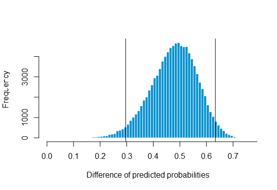
hist(res)

mean(res)

[1] 0.4781587

quantile(res, c(0.025, 0.975))

     2.5%     97.5%
0.2961805 0.6334994

Based on this simulation using $100\,000$ random draws, the difference of predicted probabilities is $0.478$ with a corresponding 95% confidence interval of $(0.296; 0.633)$. This is similar to the other answers.
The package clarify simplifies these steps greatly. Here is it in action (output is not shown):
library(MASS)
library(clarify)

set.seed(1234)

x <- runif(100, 0, 1)
y <- rbinom(100, size=1, prob = x)

model <- glm(y ~ x, family = binomial("logit"))

# Simulate coefficients from the model
s <- sim(model, n = 1e4)

# Define the function that calculates the difference between the predicted probabilities
my_fun <- function(fit) {
  predict(fit, newdata = data.frame(x = 0.75), type = "response") - predict(fit, newdata = data.frame(x = 0.25), type = "response")
}

# Apply the function to the simulated coefficients earlier
est1 <- sim_apply(s, FUN = my_fun)

# Plot and summaries the results
plot(est1, method = "quantile", reference = TRUE)
summary(est1, ci = TRUE, level = 0.95, method = "quantile")
Method: Parametric bootstrap
A parametric bootsrap confidence interval can be calculated using the following steps (Adjei & Karim 2016):
- Estimate the model and store the predicted probabilities $\hat{\pi}_i$.
- Draw a bootstrap sample $(x, y^{*})$ where $y^{*}_i=\operatorname{Ber}(\hat{\pi}_i)$.
- Fit the model with the data obtained in step 2.
- Estimate the difference in predicted probabilities from model in step 3 and store them.
- Repeat steps 2-4 a large number of times.
- Summarize the stored differences.
Again in R:
set.seed(1234)

x <- runif(100, 0, 1)
y <- rbinom(100, size = 1, prob = x)

model <- glm(y ~ x, family = binomial("logit"))

pihat <- predict(model, type = "response")

param_boot <- replicate(1e4, {
  ystar <- rbinom(100, 1, prob = pihat)
  mod <- glm(ystar~x, family = binomial)
  c(plogis(matrix(c(1, 0.75), ncol = 2) %*% matrix(coef(mod))) - plogis(matrix(c(1, 0.25), ncol = 2) %*% matrix(coef(mod))))
})

mean(param_boot)

[1] 0.4903014

quantile(param_boot, c(0.025, 0.975))

     2.5%     97.5%
0.3185213 0.6580579
Based on this simulation using $10\,000$ replications, the difference of predicted probabilities is $0.49$ with a corresponding 95% confidence interval of $(0.319; 0.658)$.
Method: Nonaparametric bootstrap
A nonparametric bootsrap confidence interval can be calculated using the following steps (Adjei & Karim 2016, see also my answer here):
- Draw $n$ observations from the original dataset of size $n$ with replacement.
- Fit the model using the data obtained in step 1.
- Estimate the difference in predicted probabilities from model in step 2 and store them.
- Repeat steps 1-3 a large number of times.
- Summarize the stored differences.
Here's how you could do it in R:
set.seed(1234)

x <- runif(100, 0, 1)
y <- rbinom(100, size = 1, prob = x)

dat <- data.frame(x, y)

nonparam_boot <- replicate(1e4, {
  mod <- glm(y~x, family = binomial, data = dat[sample.int(100, replace = TRUE), ])
  c(plogis(matrix(c(1, 0.75), ncol = 2) %*% matrix(coef(mod))) - plogis(matrix(c(1, 0.25), ncol = 2) %*% matrix(coef(mod))))
})

mean(nonparam_boot)

[1] 0.4906483

quantile(nonparam_boot, c(0.025, 0.975))

     2.5%     97.5%
0.3266630 0.6551795
Based on the nonparametric bootstrap using $10\,000$ replications, the difference of predicted probabilities is $0.49$ with a corresponding 95% confidence interval of $(0.327; 0.655)$.
References
Adjei, I. A., & Karim, R. (2016). An application of bootstrapping in logistic regression model. Open Access Library Journal, 3(9), 1-9.
Carsey, T. M., & Harden, J. J. (2013). Monte Carlo simulation and resampling methods for social science. Sage Publications.
King, G., Tomz, M., & Wittenberg, J. (2000). Making the most of statistical analyses: Improving interpretation and presentation. American journal of political science, 347-361.


errbar? $\endgroup$