Interpretation of Eigenvalue vs. Singular Value plot

Question

I'm doing some preliminary analysis on the feature matrix for a certain dataset (rows are observations, columns are feature dimensions).

I have computed the SVD and PCA decompositions for this matrix using the below python code;

# SVD decomposition
u, s, v = np.linalg.svd(mdl.feature_mat, full_matrices=False)

# PCA decomposition
covmat = mdl.feature_mat.T.dot(mdl.feature_mat)
evs, evmat = np.linalg.eig(covmat)

I then plotted the (sorted descending) relative magnitudes of the singular/eigen values. This gives me the following plot;

Clearly, many of the features in this matrix are redundant, and the signal (if any) is being carried by only a few orthogonal dimensions. My question is this;

How am I to interpret the fact that the relative singular value magnitudes have a wider tail than the relative eigenvalue magnitudes?

What is the physical interpretation / difference between singular and eigen-values?

Answer 1

There are many ways to obtain the eigenvalues and eigenvectors of a real, square, symmetric correlation (covariance) matrix $\mathbf{R}$, and SVD is one way. After you obtain eigenvalues and eigenvectors (from what ever method you want), you then use PCA for obtaining the orthogonal projection. [Factor analysis (FA) is similar to PCA, but has an infinitely large number of solutions, and in fact, PCA is the "principal component solution to the factor analysis problem"].

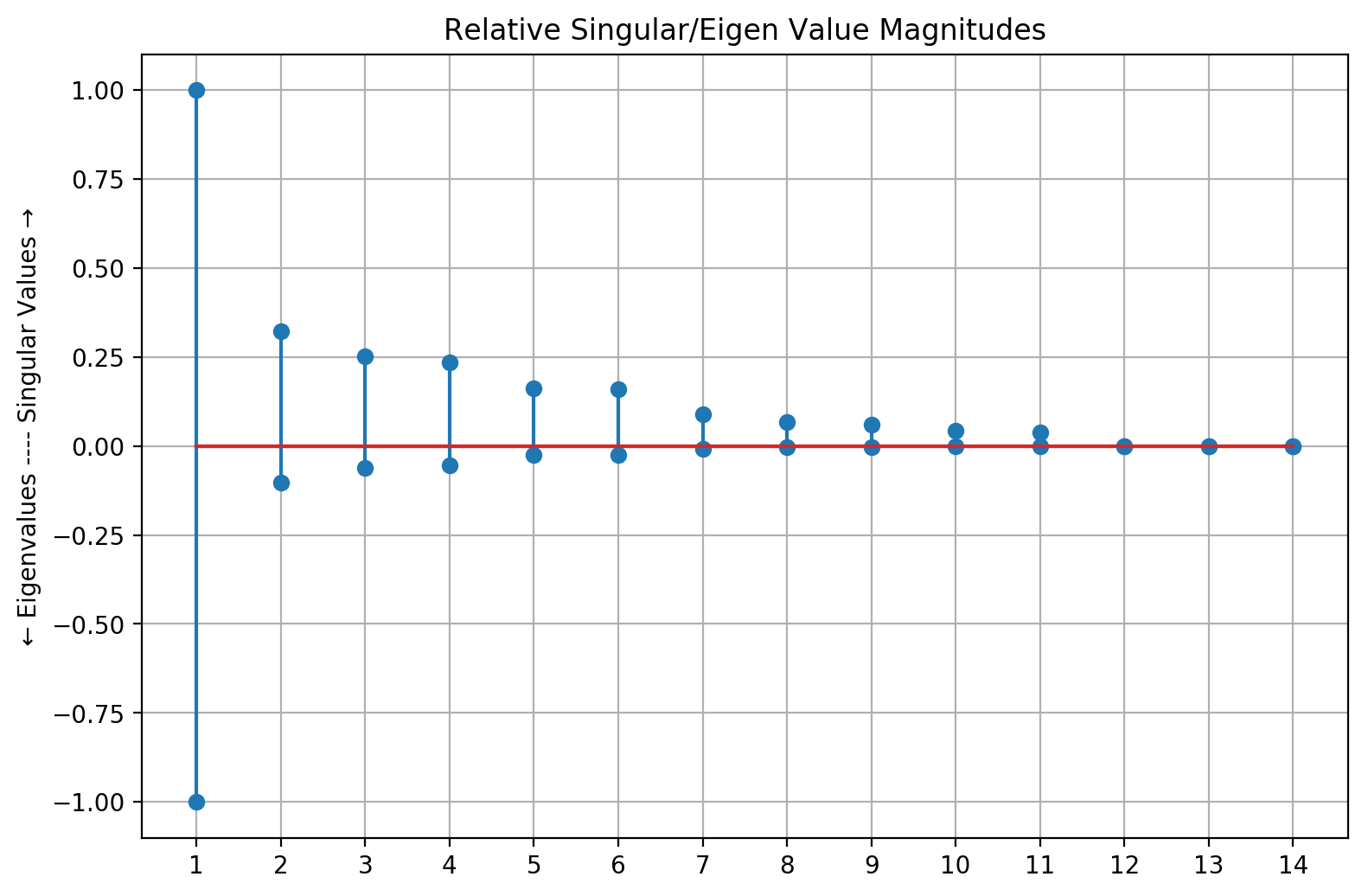
The eigenvalues $\lambda_1 \geq \lambda_2 \geq \cdots \lambda_p$ for a positive definite, $\mathbf{R}\succ 0$, correlation matrix $\mathbf{R}$ are all greater than zero, and eigenvalues for a positive semi-definite, $\mathbf{R}\succeq 0$ are greater than or equal to zero. Since 3 of your 14 eigenvalues are zero, your $\mathbf{R}$ matrix is positive semi-definite, suggesting 3 features are perfectly correlated ($r=1$) with one another, so they are redundant. You therefore need to identify which of the features have perfect correlation, and drop the redundant ones leaving only one feature out of the set of redundant features.

I wouldn't recommend re-scaling eigenvalues so the greatest (principal) is one. Rather, I always use $\mathbf{R}$ for which the sum of the eigenvalues is equal to the number of features, $\sum_j^p \lambda_j =p$, and then I can easily gauge how many features load together. (if you use the covariance matrix $\mathbf{C}$ for PCA, the eigenvalues don't sum to $p$).

The sum of your singular values from 2-14 looks about one, and since your $\lambda_1=1$, my guess is that about 7 features are highly correlated with each other, 3-4 are orthogonal to all other features (near-zero correlation), and 3 are perfectly correlated with one another -- which are causing your zero eigenvalues.

The above is for the "symmetric eigenvalue problem", i.e., using a real, square, symmetric matrix like $\mathbf{R}$ or $\mathbf{C}$. Hopefully, you didn't run SVD and PCA on the $n \times p$ data matrix $\mathbf{X}$ did you? That would be the "non-symmetric eigenvalue problem," for which the above descriptions and rules don't hold.