Updating Prediction Errors in Gradient Ascent (Friston's Free-energy)

Question

Background

In Rafal Bogacz's tutorial on the free-energy framework for modelling perception and learning, section 2.3 we have:

$$\dot{\phi} = \frac{\partial F}{\partial\phi} = \varepsilon_u g'(\phi) - \varepsilon_p \tag{9 & 12}$$

$\dot{\phi}$ is the rate of change of $\phi$ with time, and used in gradient accent to update $\phi$.

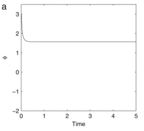
Here's the MathLab code, and the result:

So far so good.

Updating prediction errors

The equation above include two variables, both express prediction errors. Here's one of them:

$$\varepsilon_p = \frac{\phi - Vp}{\mathit{\Sigma}_p} \tag{10}$$

And it is obvious that this can be rearranged like so:

$$0 = \phi - Vp - \mathit{\Sigma}_p \varepsilon_p$$

Now I can only assume that because neural circuits can't do division, the equation above also gets updated in the gradient ascent. The update given is (MathLab code):

$$\dot{\varepsilon_p} = \phi - Vp - \mathit{\Sigma}_p \varepsilon_p \tag{13}$$

And it goes:

It is easy to show that the nodes with dynamics described by Eqs. (13)–(14) converge to the values defined in Eqs. (10)–(11). Once Eqs. (13)–(14) converge, then $\dot{\varepsilon}=0$, so setting $\dot{\varepsilon}=0$ and solving Eqs. (13)–(14) for ${\varepsilon}$, one obtains Eqs. (10)–(11).

Now give me 500 years and I wouldn't come up with this solution (definitely not after 120 years). Is this some common knowledge I've been missing, or is it a unique treatment? Where can I read more about these sorts of 'dynamics'?

What's more, despite understanding the $\dot{\varepsilon}=0$ case, I don't really get why or how this works. Namely, In (10) we divide by $\mathit{\Sigma}_p$ whereas in (13) we multiply.

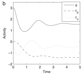
Another issue is that if you look at the plot, you'll see that neither prediction errors actually converge to 0:

So can someone please provide a layperson explanation as to how (13) works? Maybe by using a simple case?

Answer 1

OK, I've worked it out. Here's the most trivial example I could think of.

$$ I = \frac{V}{R}$$

which can be rearranged:

$$ IR = V$$

So in:

$$ \dot{I} = V - IR$$

$V$ stands for the the actual voltage, where $IR$ stand for the calculated voltage based on parameter $I$. The difference between them is the error.

MathLab:

voltage = 10;
resistance = 5;
current(1) = 0; % What we're after. As current = voltage / resistance, it's 2.

DT = 0.01;
MAXT = 1;

for t = 2:MAXT/DT
    error = voltage - resistance * current(t-1);
    current(t) = current(t-1) + DT * error;
end

plot([DT:DT:MAXT], current);
xlabel('Time');
ylabel('current');

And the graph: