Calculating Confidence Intervals when proportion is skewed [duplicate]

Question

I have 15,000 address strings which I have written a piece of code which assigns them to broad geographic region e.g. American address assigned to North America. I would like to check the accuracy of my code. However I must manually check the strings. To do this I've taken a sample (SRS). I set a margin of error of 5%, a CI of 95% and a response distribution of 50%. Therefore, I assumed that I would assign the correct region half the time.

The issue here is that I am much more accurate then I anticipated. Of my sample of 375,372 (99%) were assigned to the correct location. This means I am unable to calculate lower and upper confidence limits.

Is there any other types of formula I could use when your response distribution is skewed to a highly positive outcome? Or is the only remedy to simply increase my sample size?

Answer 1

A quick answer based on the links (and corresponding references) in Comments: Use a Bayesian probability interval (based on a uniform prior) to serve as a frequentist confidence interval (CI).

If you have $X = 3$ successes in $n = 275$ trials, then your 95% CI can be found in R as qbeta(c(.025, .975), x + 1, n - x + 1):

x = 3;  n = 275
qbeta(c(.025,.975), x+1, n-x+1)
[1] 0.003962534 0.031435106

So you might use $(0.004,\,0.031)$ as your 95% CI.

Notes: (a) The Jeffrey's interval mentioned in references uses 0.5 where I have used 1. That is

 x = 3;  n = 275
 qbeta(c(.025,.975), x+.5, n-x+.5)
 [1] 0.003081784 0.028823996

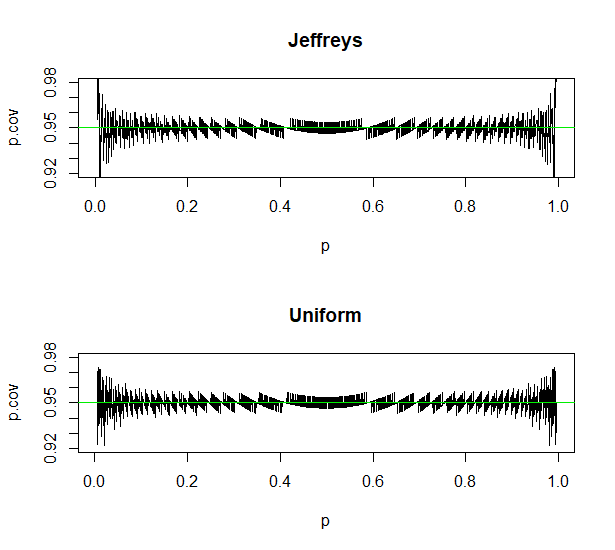
Most of the time, the two intervals are almost the same. In my experience, using the uniform prior instead of the Jeffreys prior happens to give slightly more consistent coverage probabilities in some cases of proportions very near 0 or 1. Plots of coverage probabilities for $n = 275$ are shown below:

(b) If you're using software other than R, qbeta is the an inverse CDF function (quantile function) for a beta random variable. Most commercial programs can be used to get the same result (even if not as compactly as R). For example, using Minitab we get:

MTB > invcdf .025;
SUBC> beta 4 273.

Inverse Cumulative Distribution Function 
Beta with first shape parameter = 4 and second = 273
P( X ≤ x )          x
     0.025  0.0039625

MTB > invcdf .975;
SUBC> beta 4 273.

Inverse Cumulative Distribution Function 
Beta with first shape parameter = 4 and second = 273
P( X ≤ x )          x
     0.975  0.0314351