Interpretation of functional regression models for scalar response

Question

I have an application scenario in which I want to determine a single outcome from the course of a series of measurements. I decided to give functional regression a try, so I read and ran the example from chapter 9 of Ramsay's Functional Data Analysis with R and MATLAB, where the annual precipitation is modelled using the daily temperature curves of Canadian weather stations.

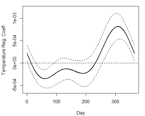
Fig 9.3 on page 139 shows the regression coefficients $\beta(t)$:

At the moment, my interpretation of this is that high temperature has a negative effect on precipitation early in the year and a positive effect at the end.

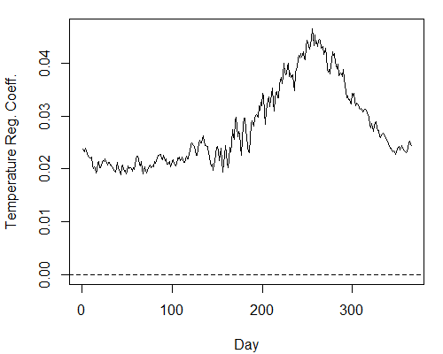
Unfortunately, however, I was somehow unable to find enough information to convince myself that this is truly the right way to interpret $\beta(t)$, so I played around with the data and tracked the regression slopes of a series of separate linear regression models, one for each day:

While rise and fall of the coefficients in the second half of the year are also visible this way, the estimates never become negative or even close to zero.

As a result, I am now more confused than before. So my questions are:

What am I missing? Have I perhaps completely misunderstood the way functional covariates work?

Thank you very much in advance!

---

R-Code to reproduce the plots:

library(fda.usc)

annualprec = log10(apply(daily$precav,2,sum))

tempbasis =create.fourier.basis(c(0,365),65)
tempSmooth=smooth.basis(day.5,daily$tempav,tempbasis)
tempfd =tempSmooth$fd

templist = vector("list",2)
templist[[1]] = rep(1,35)
templist[[2]] = tempfd

conbasis = create.constant.basis(c(0,365))

Lcoef = c(0,(2*pi/365)^2,0)
harmaccelLfd = vec2Lfd(Lcoef, c(0,365))
lambda = 10^12.5
betabasis = create.fourier.basis(c(0, 365), 35)

betafdPar = fdPar(betabasis, harmaccelLfd, lambda)

betalist = vector("list",2)
betalist[[1]] = conbasis
betalist[[2]] = betafdPar

fRegressList = fRegress(annualprec,templist,betalist)

annualprechat = fRegressList$yhatfdobj
resid = annualprec - annualprechat
SigmaE.= sum(resid^2)/(35-fRegressList$df)
SigmaE = SigmaE.*diag(rep(1,35))
y2cMap = tempSmooth$y2cMap
stderrList = fRegress.stderr(fRegressList, y2cMap,SigmaE)

betaestlist = fRegressList$betaestlist
betafdPar = betaestlist[[2]]
betafd = betafdPar$fd
betastderrList = stderrList$betastderrlist
betastderrfd = betastderrList[[2]]
par(mar=c(4,4,1,1)+.1)
plot(betafd, xlab="Day",ylab="Temperature Reg. Coeff.",
     ylim=c(-6e-4,1.2e-03), lwd=2)
lines(betafd+2*betastderrfd, lty=2, lwd=1)
lines(betafd-2*betastderrfd, lty=2, lwd=1)

###

lm.series <- sapply(1:nrow(daily$tempav),function(x){
  coef(lm(annualprec~1+daily$tempav[x,]))
})
plot(t(lm.series)[,2],t="l",ylim=c(0,max(lm.series[2,])),
     xlab="Day",ylab="Temperature Reg. Coeff.")
abline(h=0,lty=2)

Answer 1

This is the right way to interpret the functional linear model although you should be careful for the months where 0 is contained in the confidence bands. This interpretation is explained in page 257 of Functional Data Analysis by Ramsay and Silverman (2nd edition) with this example.

The problem of fitting a univariate linear model for each day is that you are falling for omitted variable bias. This problem arise when your omitted covariates are correlated. This is the usual case for functional data (the temperature of one day is strongly correlated with the following and previous ones) and is one of the first motivations for using a functional models when covariates altough discrete may be represented as functional.