Statistically significant difference between distributions only knowing the mean and std dev?

Question

I have 3 specimens (A, B & C) and 5 sets of observations from A & B but only 4 from C.

Each set of observations has been reported as a mean & a standard deviation. I do not have access to the underlying data.

A:
0.230, 0.104
0.245, 0.117
0.223, 0.098
0.246, 0.131
0.240, 0.135

B:
0.225, 0.121
0.218, 0.111
0.224, 0.125
0.231, 0.129
0.204, 0.092

C:
0.245, 0.14
0.225, 0.09
0.249, 0.104
0.229, 0.099

I am curious about whether the samples are statistically different from each other as far as this measurement is concerned.

My initial attempt was just to use the means so I did some T tests between them & then an ANOVA on all 3 using Python & Scipy's stats library.

import numpy as np
import scipy.stats as stats

A = np.array([0.230, 0.245, 0.223, 0.246, 0.240])
B = np.array([0.225, 0.218, 0.224, 0.231, 0.204])
C = np.array([0.245, 0.225, 0.249, 0.229])

AB_ttest  = stats.ttest_ind(A, B)
AC_ttest  = stats.ttest_ind(A, C)
BC_ttest  = stats.ttest_ind(B, C)

ABC_anova = stats.f_oneway(A, B, C)

print("A, B T test: ", AB_ttest)
print("A, C T test: ", AC_ttest)
print("B, C T test: ", BC_ttest)
print(" ")
print("ANOVA: ", ABC_anova)

Here's the results rounded to 3 decimal places...

A, B T test:  statistic = 2.561,  p value = 0.0336
A, C T test:  statistic = -0.028, p value = 0.978
B, C T test:  statistic = -2.263, p value = 0.058

ANOVA:  statistic = 3.889, p value = 0.0528

OK so here's where I realize I dont know what's going on.

Given that p < 0.05 implies a statitically significant difference (ssd) then the T test for A & B suggests such a difference and yet the ANOVA suggets that there is no ssd between them? Or am I reading this all wrong?

Also I'm not convinced that my approach is an acceptable statitical anlysis of this kind of data . If not how should I be approaching this?

Answer 1

We must assume these "standard deviations" are actually standard errors of the mean (which is likely), for otherwise they are worthless without counts of the raw data used to compute each standard deviation. (If these are truly standard deviations but all those counts are known to be the same, then you don't need to know the common count because the weights, as described below, depend only on the relative counts, and you may proceed as if they are standard errors.)

These standard errors (SEs) do not vary a great amount (the square of the largest is only about twice the square of the smallest), so it's likely they won't make a difference: you can use standard Analysis of Variance (ANOVA).

ANOVA is a good approach. It is Ordinary Least Squares (OLS) regression in disguise. This insight permits you to use weighted OLS to handle the information conveyed by the SEs. The proper way to weight the observations is proportional to the reciprocal variance: that is, to the reciprocal squared SEs: see https://stats.stackexchange.com/a/246449/919 and https://stats.stackexchange.com/a/12255/919 for the mathematics behind this.

In R, for instance, after creating a data frame X with Value, SE, and Group fields, you could use its OLS procedure lm:

fit.w <- lm(Value ~ Group, X, weights = 1/X$SE^2)
summary(fit.w)

Using group $B$ as the reference, the output for your data is

Coefficients:
            Estimate Std. Error t value Pr(>|t|)    
(Intercept)  2.17973    0.05081  42.902 1.34e-13 ***
GroupA       0.16855    0.07227   2.332   0.0397 *  
GroupC       0.16913    0.07295   2.318   0.0407 *  
---
Signif. codes:  0 ‘***’ 0.001 ‘**’ 0.01 ‘*’ 0.05 ‘.’ 0.1 ‘ ’ 1

Residual standard error: 0.1006 on 11 degrees of freedom
Multiple R-squared:  0.3976,  Adjusted R-squared:  0.2881 
F-statistic:  3.63 on 2 and 11 DF,  p-value: 0.06157

Pay no attention to the individual p-values (in the right hand column). They are deceptively low because you plan to make three related tests, not one; and these p-values are computed only for the case where each of the coefficients they test is the only one you are interested in. (By the way, the unweighted fit produces slightly lower p-values, but not enough to make us analyze the effects of the weights in more detail.)

The first result to examine is the p-value for the overall regression F-statistic, reported at the very end as $0.06157.$ That's weak evidence of any difference. Many people would stop here and treat the groups as having equal means. But if you can accept such weak evidence (for instance, your threshold might be $10\%$ rather than $5\%$), you would proceed (as usual) to make post hoc comparisons. You need to account for planning on three tests.

For instance, you could use Tukey's HSD to perform the three comparisons among the groups.

TukeyHSD(aov(fit.w))

             diff         lwr        upr     p adj
B-A -0.1685526460 -0.35444973 0.01734443 0.0764764
C-A  0.0005789762 -0.19659465 0.19775261 0.9999653
C-B  0.1691316222 -0.02804201 0.36630525 0.0951872

Again, you would begin your review by consulting the "adjusted p-values" in the rightmost column. Two of them are less than $0.10,$ but none are less than $0.05.$ If your threshold for statistical significance is $0.10,$ for instance, then you would conclude there are differences between groups $A$ and $B$ (first line, $p=0.076$) and groups $C$ and $B$ (third line, $p=0.095$), but not between groups $C$ and $A$ (which exhibit very nearly the same weighted mean).

Answer 2

1

You need to know more than just the mean and std dev (and also standard deviation is ambigious. See 1 2)

Statistically significant difference between distributions only knowing the mean and std dev?

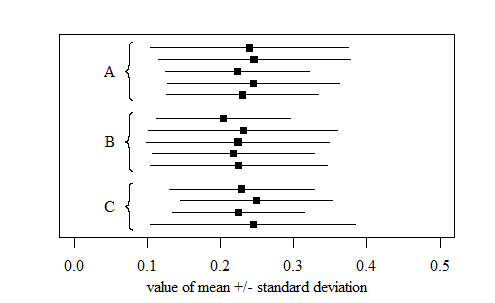
I have placed your data in a graph to show a bit better what we are dealing with:

I note two strange aspects:

• I wonder whether the reported values are standard errors. It does not make sense that the reported standard errors (which should relate to the standard deviation of the sample distribution of the means) is roughly $0.1$ while the standard deviation of the sampled means is $\ll 0.1$ ?

• You state that the sample size of each case is around $10^6$ to $10^7$. But in that case it would be very strange to interpret the values around $0.1$ as standard errors, because they would be very large. They are more likely to be standard deviation of the group/population. But, when they are the standard deviations then the standard error would be very small (scaling by $n^{-0.5}$) and then the observed between-groups variance/deviation is larger than what one would expect from the error of measurement.

  It could be that this is a mixed model where the means of the groups are not to be considered the same for each experiment but instead are to be considered to be sampled from some distribution.

  Whether you are dealing with a Gaussian distribution is not clear from the current context, which makes it difficult to blindly apply ANOVA, but anyway when you do wish to model this as ANOVA, which is indirectly some linear model, then you will need to consider each of the 14 measured means to be sampled from a distribution with a different variance/deviation. The distributions will have the same mean, if the null hypothesis is correct, but they will not have the same variance.

  When you are dealing with samples $X_i \sim N(\mu,\sigma_i^2)$ where $\sigma_i$ is variable (different for each experiment/sampled mean $i$) and relates to the variance $\sigma^2$ of the true means and the error $\epsilon_i$ of the measurement/sampling of the means ($\sigma_i = \sqrt{\sigma + \epsilon_i}$), then the likelihood function will be like:

  $$\log(\mathcal{L}) = - \frac{n}{2} \log(2\pi) - \frac{n}{2} \log(\sigma + \epsilon_i^2) + \sum \frac{(\mu_i-\mu)^2}{2(\sigma^2+\epsilon_i^2)}$$

  The problem in your situation is that you do not know $\epsilon_i$ (which is not just based on the standard deviation, but also on the sample size). But when you approximate all the $\epsilon_i$ to be the same then the above becomes just like a regular least squares fit and you can use ANOVA in the typical way.

To continue with your data you should clear up what the deviations refer to and what the different sample sizes are. (Although you could also assume the error in each point is similar and apply ANOVA, which will now just be not very exact in the case that in reality there are large differences in the standard errors. It depends a bit on your problem whether or not you want to be very exact or not. Does it matter to you when you obtain a p-value of 0.07 when in reality it should be 0.05?)

2

The t-test and ANOVA consider different observations as belonging to the 5% most significant(/extreme) observations.

the T test for A & B suggests such a difference and yet the ANOVA suggets that there is no ssd between them? Or am I reading this all wrong?

• First of all, it is difficult to interpret results when the underlying statistical model is not very certain.

  The mean value of B is lower than A and C, but this is mostly due to only one or two relatively low values. It is difficult to interpret this: 1) we do not know what sort of data this is 2) we can not assess whether these data are to be reasonably considered from a normal distribution (with the same variance).

  Say, when the data from group B is lower quality (e.g. smaller sample size) then it is not strange that some values will be extreme, and with only 5 measurements those extreme values might likely fall towards the same direction making you believe that the group B itself (not the measurement) is a lot different. If you would do a Kruskal-Wallis test then the p-value will be 0.1007. (this means: you need more data and information if you wish to be more sure)

• Secondly, in the difference between the p-value of the t-test and p-value of ANOVA there are two effects that play a role. 1) The t-test make multiple comparisons and these should be corrected for. 2) Even when you correct for multiple comparisons, for instance by using Tukey's HSD test then the t-test will have low p-values for different cases than the ANOVA test.

  Regarding the difference between t-test and ANOVA there have been other questions before: R Tukey HSD Anova: Anova significant, Tukey not? , How can I get a significant overall ANOVA but no significant pairwise differences with Tukey's procedure? and Significant ANOVA interaction but non-significant pairwise comparisons

  In my answer to it I generated the following plot which shows that the p-values of t-test and ANOVA discriminate different cases (although both discriminate the correct p% of all cases when the null hypothesis is true).

  Figure: The criteria for the Tukey HSD test (showing the smallest and second smallest p-values on the x- and y-axis with two vertical lines at 0.05 and 0.1) with the criteria for the F-test (the red dots have p-value below 0.05, the green dots have p-value above 0.05 and below 0.1, black dots are above 0.1).

  

  Your case is actually of the type where the smallest p-value in Tukey's test has a higher value than the p-value of the ANOVA test (because you have two values close to each other which 'benefits' ANOVA). You can also see this in the results from the answer by Whuber which shows higher p-values for Tukey's test than for the ANOVA F-test.

3

p < 0.05 implies a statitically significant difference

...

ANOVA suggets that there is no ssd between them?

I believe that you should not consider significance as a dichotomous yes/no present/absent question.

In the first place you should consider the p-value and significance just as a continuous measure that is qualifying (not quantifying) the difference between the groups and indicating how remarkable that observed difference is (remarkable in relation to the null, -no effect-, hypothesis and the probability to observe such difference or effect size).

Any boundary dividing significant and not-significant is a second thought. It is not really dividing results into significant and not-significant but instead into significant enough and not-significant enough (for whatever goal is taken into consideration).

What one should not forget is that besides significance also the effect size (is it large or small) should be taken into consideration. Whether a result (observed effects size) is important should be determined by the effect size (or cost functions) and the significance (that is, statistical significance) is only an indicator of the quality (relative accuracy) of the obtained result but not of whether or not the result is relevant or not. When the observed effect size is large enough to be of interest but you find the significance (accuracy) not sufficient then you should perform more/better observations.

4

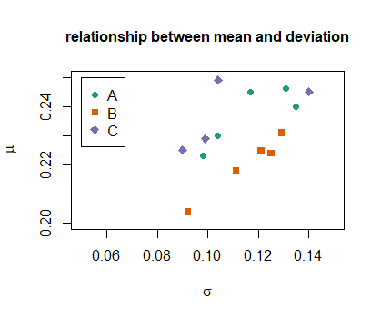
The following plot might also be of interest to you. There seems to be relationship between the observed mean and standard deviation. The deviation is larger when the mean is larger.

This indicates that you do not have a situation of ordinary (homogeneous) sampling from a normal distribution.

Answer 3

You can't do ANOVA without having the underlying data, because ANOVA requires that you compute the squared differences between each observation and its group mean.

You can't treat the means as observations, and then do ANOVA on that. You can do it procedurally, but its not meaningful.

The examples here will explain this: http://sphweb.bumc.bu.edu/otlt/MPH-Modules/BS/BS704_HypothesisTesting-ANOVA/BS704_HypothesisTesting-Anova_print.html