Terminology
The model you fitted with the lm() function in R is actually a linear regression model, not a multilevel linear regression model. In statistics, we reserve the multilevel terminology for situations where the data exhibit a natural form of nesting (e.g., students nested in schools).
Factors in R
The Smoke predictor appears to be declared as a factor in your data (i.e., a categorical variable). Moreover, R thinks this factor is unordered (i.e., its categories are NOT assumed to follow a natural ordering). You can check this with the command:
str(surveyNA$Smoke)
Dummy Variables
For the reasons described above, when you include the predictor Smoke as a factor in your model, its effect on Height will be encoded using k - 1 = 4 - 1 = 3 dummy variables, where k = 4 represents the number of categories (or levels) of Smoke. These dummy variables are denoted by R as SmokeNever, SmokeOccas and SmokeRegul. As you can see, the dummy variable SmokeHeavy was excluded from the model to avoid collinearity. You could have included this dummy variable in the model but then you would have had to exclude the intercept:
survfit0 <- lm(Height~ -1 + Smoke, data = surveyNA)
When excluding the intercept from the model, summary(survfit0) will report the estimated mean Height for each category/level of Smoke.
When including the intercept in the model, summary(survfit0) will report the difference in estimated mean Height values between each non-reference category of Smoke (in your case, Never, Occas and Regul) and the reference category of Smoke (Heavy).
Alphabetical Ordering of Factor Levels
You will notice that, unless you were explicit about which dummy variable you wanted to exclude from your model, R made that choice for you. Indeed, R will always - by default - exclude the dummy variable corresponding to the category/level of the factor of interest which appears first in an alphabetical list. If you list the categories/levels of Smoke, you will see that Heavy is the first in this alphabetical list: Heavy, Never, Occas, Regul.
More Thoughtful Ordering of Factor Levels
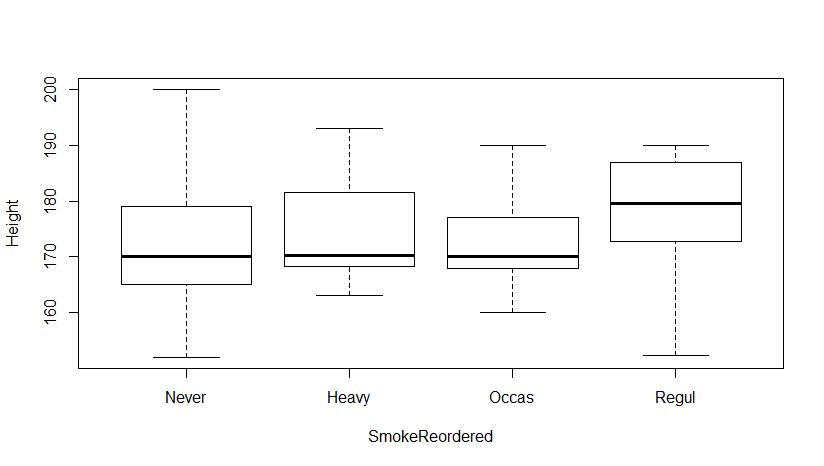
Can you override R's default? Absolutely! How you do the overriding will depend on both your research questions and your data. In this particular example, perhaps you might be interested in determining whether the mean height for the subjects you are studying tends to increase with frequency of smoking. Then you would want these dummy variables in your model: SmokeOccas, SmokeRegul, SmokeHeavy. Having these in your model would enable you to see how, compared to never smoking, the mean height goes up as you move up the ladder from one frequency of smoking to another. To fit such a model, you would have to rearrange the levels of your Smoke factor (currently listed alphabetically):
surveyNA$Smoke <- factor(surveyNA$Smoke,
                         levels = c("Never",
                                    "Occas",
                                    "Regul",
                                    "Heavy"))
However, before you fit your model with the re-arranged factor:
survfit1 <- lm(Height ~ 1 + Smoke, data = surveyNA)
there is one more thing you should do. You should check how many subjects in your data fall into each of your category of Smoke and keep an eye in particular on the reference category Never, whose dummy variable would be excluded from your current model:
table(surveyNA$Smoke)
If it turns out that your reference category, Never, has the fewest number of subjects represented in the data (much smaller than the number of subjects in all other categories), you could change your reference category to a richer category to avoid model estimation problems. This won't affect your ability to answer your research question - you'll be able to interrogate the model more after you fit it.
If it also turns out that one of the other categories (say Heavy) has only 3 subjects in it, then you could decide to merge it with its neighbouring category, Regul, to create a new category named Regul/Heavy. If you don't do this merging, the standard errors for the effect of SmokeHeavy will likely be very large, reflecting the uncertainty involved in estimating this effect with such few data points.
Impact of Re-Ordered Factor Levels
What happens to your model when you re-order the categories of Smoke so that the reference category changes?
The answer is that your model parametrization changes, which in turns impacts the inference you can conduct based on the output reported by R in the model summary.
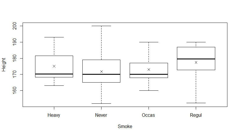
To illustrate this, assume you consider two competing models. Model 1 uses Heavy as a reference level for the Smoke predictor, while Model 2 uses Never as a reference level. The two models clearly have different formulations, as they include different dummy variables.
Model 1:
$Height = \beta_0 + \beta_1*SmokeNever + \beta_2*SmokeOccas + \beta_3*SmokeRegul + \epsilon$
Model 2:
$Height = \beta_0^* + \beta_1^**SmokeReorderedHeavy + \beta_2^**SmokeReorderedOccas + \beta_3^**SmokeReorderedRegul + \epsilon^*$
In Model 1, for the target population, the mean Height for heavy smokers is quantified by the parameter $\beta_0$, the mean Height for those who never smoke is quantified by the parameter $\beta_0 + \beta_1$, the mean Height of occasional smokers is quantified by the parameter $\beta_0 + \beta_2$ and the mean Height for regular smokers is quantified by the parameter $\beta_0 + \beta_3$. In the summary for Model 1, R will report estimated values for the parameters $\beta_0$, $\beta_1$, $\beta_2$ and $\beta_3$, along with tests of hypotheses of the form:
- Ho: $\beta_0 = 0$ versus Ha: $\beta_0 \neq 0$;
- Ho: $\beta_1 = 0$ versus Ha: $\beta_1 \neq 0$;
- Ho: $\beta_2 = 0$ versus Ha: $\beta_2 \neq 0$;
- Ho: $\beta_3 = 0$ versus Ha: $\beta_3 \neq 0$.
In other words, R will estimate the mean value of Height for heavy smokers (quantified by $\beta_0$) and test whether it is different from 0. It will also (i) estimate the difference in mean Height values between those who never smoke and heavy smokers (quantified by $\beta_1$) and test whether this difference is different from 0, (ii) estimate the difference in mean Height values between those who occasionally smoke and heavy smokers (quantified by $\beta_2$) and test whether it is different from 0 and (iii) estimate the difference in mean Height values between those who regularly smoke and heavy smokers (quantified by $\beta_3$) and test whether it is different from 0.
In Model 2, the mean Height for those who never smoke is quantified by the parameter $\beta_0^*$, the mean Height for those who are heavy smokers is quantified by the parameter $\beta_0^*+ \beta_1^*$, the mean Height of occasional smokers is quantified by the parameter $\beta_0^* + \beta_2^*$ and the mean Height for regular smokers is quantified by the parameter $\beta_0^* + \beta_3^*$. In the summary for Model 2, R will report estimated values for the parameters $\beta_0*$, $\beta_1^*$, $\beta_2^*$ and $\beta_3^*$, along with tests of hypotheses of the form:
- Ho: $\beta_0^* = 0$ versus Ha: $\beta_0^* \neq 0$;
- Ho: $\beta_1^* = 0$ versus Ha: $\beta_1^* \neq 0$;
- Ho: $\beta_2^* = 0$ versus Ha: $\beta_2^* \neq 0$;
- Ho: $\beta_3^* = 0$ versus Ha: $\beta_3^* \neq 0$.
Thus, for Model 2, R will estimate the mean value of Height for those who never smoke (quantified by $\beta_0^*$) and test whether it is different from 0. It will also (i) estimate the difference in mean Height values between heavy smokers and those who never smoke (quantified by $\beta_1^*$) and test whether it is different from 0, (ii) estimate the difference in mean Height values between those who occasionally smoke and those who never smoke (quantified by $\beta_2^*$) and test whether it is different from 0 and (iii) estimate the difference in mean Height values between those who regularly smoke and those who never smoker (quantified by $\beta_3^*$) and test whether it is different from 0.
This is the reason why I added my comment to this answer:
When you look at the significance of REGULAR in a model where HEAVY is treated as the reference, you are testing for a difference in the mean Height between subjects in your target population who are REGULAR smokers and those who are HEAVY smokers. When you look at the significance of REGULAR in a model where NEVER is treated as the reference, you are testing for a difference in the mean Height between subjects in your target population who are REGULAR smokers and those who are not smokers.
No wonder you get different p-values - you are performing different tests of hypotheses based on your choice of reference level!
However, as pointed out by @whuber in his comment, changing the model parametrization will not impact the estimated mean Height values for the four categories of Smoke reported by R. That is because:
$\beta_0$ in Model 1 and $\beta_0^*+ \beta_1^*$ in Model 2 are different parametrizations for the same thing, namely the mean Height of heavy smokers in the target population;
$\beta_0 + \beta_1$ in Model 1 and $\beta_0^*$ in Model 2 are different parametrizations for the same thing, namely the mean Height of those who never smoke in the target population;
$\beta_0 + \beta_2$ in Model 1 and $\beta_0^*+ \beta_2^*$ in Model 2 are different parametrizations for the same thing, namely the mean Height of occasional smokers in the target population;
$\beta_0 + \beta_3$ in Model 1 and $\beta_0^*+ \beta_3^*$ in Model 2 are different parametrizations for the same thing, namely the mean Height of regular smokers in the target population.


