Generate random samples from $f(x) \propto [1 + \sin^2(3 x)] [ 1+ \cos^4(5x)] e^{-x^2/2}$ using slice sampler

Question

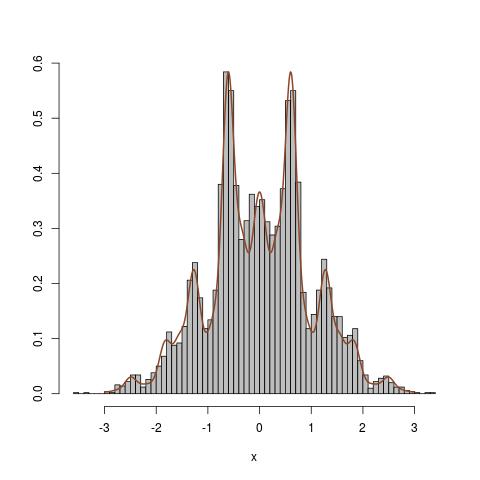
I am trying to understanding the Example 8.3 of Monte Carlo Statistical Methods from Robert and Casella. The example shows how to generate from the density $$f(x) \propto [1 + \sin^2(3x)] [ 1+ \cos^4(5x)] e^{-x^2/2}$$ using slice sampler.

Example 8.3 Consider the density proportional to $$ (1+\sin^2(3x))\,(1+\cos^4(5x))\,\exp\{-x^2/2\}. $$ The corresponding functions are, for instance, $f_1(x)=(1+\sin^2(3x))$, $f_2(x)=(1+\cos^2(5x))$, and $f_3(x)=\exp\{-x^2/2\}$. In an iteration of the slice sampler, three uniform $\mathcal U([0,1])$ $u_1,u_2,u_3$ are generated and the new value of $x$ is uniformly distributed over the set $$ \left\{ x:\, |x| \le \sqrt{-2\log\omega_3}\right\} \cap \left\{ x:\, \sin^2(3x) \ge 1-\omega_1 \right\} \cap \left\{ x:\, \cos^4(5x) \ge 1-\omega_2 \right\} \,, $$ which is made of one or several intervals depending on whether $\omega_1=u_1 f_1(x)$ and $\omega_2=u_2 f_2(x)$ are larger than $1$.

My doubth is how can I generate an uniform distribution over the set $A$?

I am using the following R code, but the result is not the expected one when comparing theoretical and empirical distributions.

f1 = function(x) 1 + sin(3 * x)^2
f2 = function(x) 1 + cos(5 * x)^4
f3 = function(x) exp(- x^2 / 2)

xs = seq(-3, 3, l = 10000)
x = c()
x0 = 0
for(j in 1:5000)
{
  cat(j, "\n")
  w1 = runif(1, 0, f1(x0))
  w2 = runif(1, 0, f2(x0))
  w3 = runif(1, 0, f3(x0))

  A1 = ifelse(w1 < 1, NaN, sample(xs[f1(xs) >= w1], 1))
  A2 = ifelse(w2 < 1, NaN, sample(xs[f2(xs) >= w2], 1))

  i3 = max(-3, -sqrt(-2 * log(w3)))
  s3 = min(sqrt(-2 * log(w3)), 3)
  A3 = runif(1, i3, s3)

  At = c(A1, A2, A3)
  At = At[!is.na(At)]

  x[j] = sample(At, 1)

  x0 = x[j]

}

fx_propto <- function(x) (1 + sin(3 * x)^2) * ( 1 + cos(5 * x)^4) * exp(-x^2 / 2)
fx <- function(x)
{
  const = integrate(fx_propto, -3, 3)$value
  fx_propto(x) / const
}

fdens = sapply(xs, fx)
hist(x, breaks = 100, probability = T)
lines(xs, fdens, col = "blue", type = "l")

Obs.: I truncated the distribution on $[-3, 3]$.

Answer 1

Debugging: In your R code, you generate three Uniforms over the three component sets of $A$ and pick one of the three at random: there is no reason for this outcome to (i) belong to $A$ and (ii) to be uniformly distributed over $A$.

Here is the R code that we used for this example, verbatim:

x<-rep(0,5000)
for (i in 2:5000){
  omega1<-(1+sin(3*x[i-1])^2)*runif(1)-1
  omega2<-(1+cos(5*x[i-1])^4)*runif(1)-1
  omega3<-sqrt(-2*log( runif(1)*exp(-x[i-1]^2/2)))
  repeat{
      y<--omega3+2*omega3*runif(1)
      if ((sin(3*y)^2>omega1)&&(cos(5*y)^4>omega2)) break
      }
  x[i]<-y
  }
plo<-hist(x,nclass=75,col="grey",proba=T,xlab="x",ylab="",main="")
labs<-seq(-3,3,.01)
dense<-(1+sin(3*labs)^2)*(1+cos(5*labs)^4)*exp(-labs^2/2)
dense<-dense*max(plo$density)/max(dense)
lines(labs,dense,col="sienna4",lwd=2)

returning the following graph (as in the book):

The explanation for the R code being justified as a Uniform simulation over $A$ is that we simulate uniformly over the component set $$A_3=\left\{x:\ |x| \leq \sqrt{-2 \log w_3 } \right\}$$ namely

y<--omega3+2*omega3*runif(1)

until the outcome belongs to $A$:

if ((sin(3*y)^2>omega1)&&(cos(5*y)^4>omega2)) break

which is a rudimentary form of accept-reject since $A\subset A_3$.