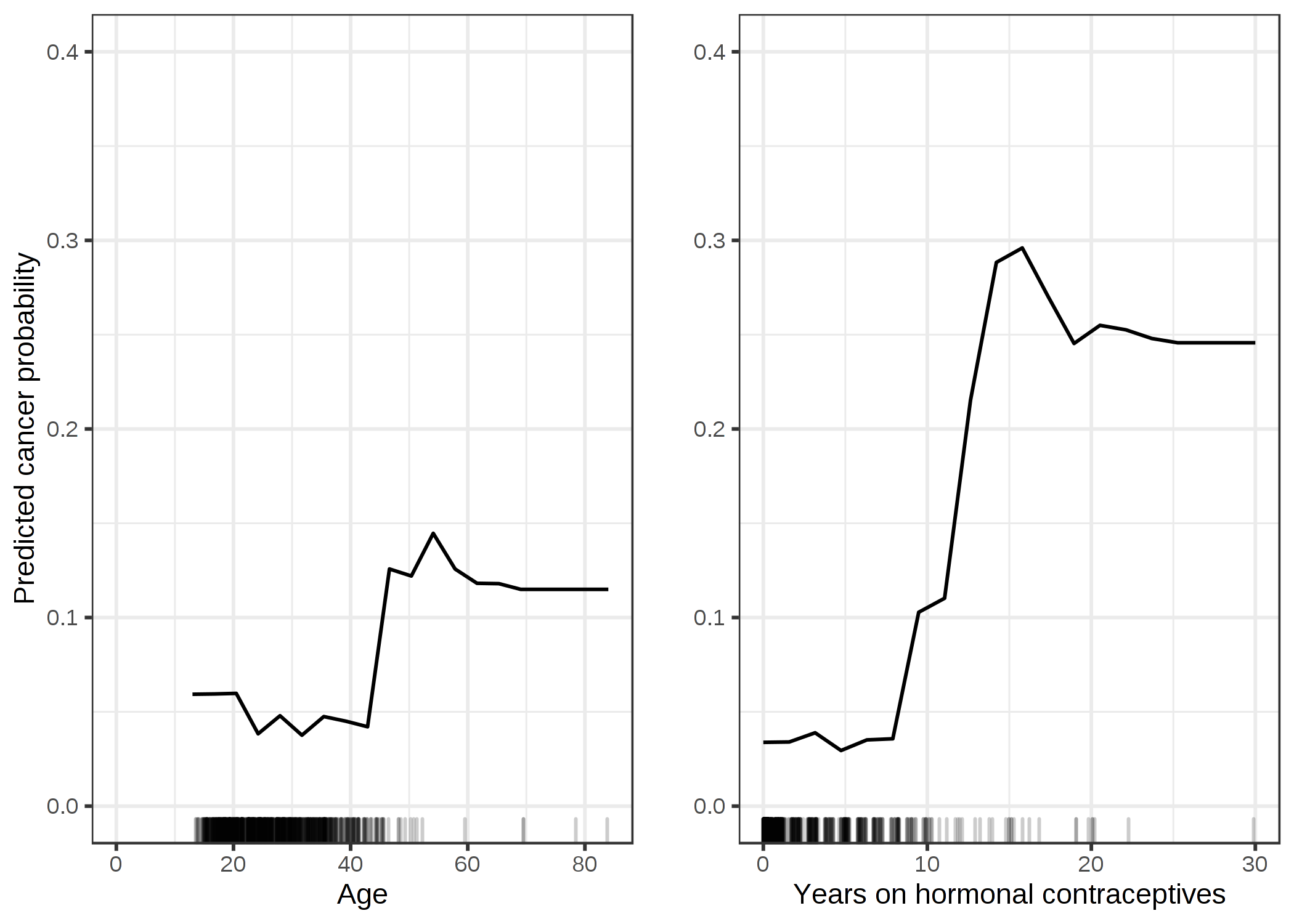
Part of what you want can be achieved through the use of partial-dependence plots (PDP) for the "important" features $x_A, \dots, x_Z$ used within the model $M$. Partial dependence plots show the average relationship between a given feature $x_A$ and the response $y$ within the fixed, joint distribution of all the other inputs $x_B, \dots, x_Z$. Particularly for a probability estimation task as the one described one can plot in each case how the final probability of death is affected. (eg. "values of systolic BP above a threshold $z$ are associated with approximately $0.40$ probability of death while below are generally $0.15$", etc.) It is notable thought that the idea of a dichotomising a continious variable is very often problematic. I would suggest presenting the whole range of a feature to describe its association with the response variable rather than focusing on a potentially arbitrary threshold.
Here is an image from the Partial Dependence Plot (PDP) of the excellent Interpretable Machine Learning e-book by C. Molnar showing what I describe above:

Note that what is an "important feature" is a bit of a "how long is a piece of string" question itself; feature importance in a GBDT can be defined with multiple ways (e.g. how many times a feature is used for splitting, what is the average cost reduction observed after splitting that feature, what is the mean SHAP value associated with that feature, what is the feature's permutation importance, etc. etc.)
Both R and Python has a number of partial dependence plot functionality. R has two great packages on that matter pdp and iml. Python has package like pdpBOX but actually since version 0.22 sklearn also supports PDPs.
Anecdotal note: I have found the insights of PDPs to be quite close to those I would get from GAMs. This is not very surprising as the use of a "penalised spline" to encapsulate non-linear relations between an explanatory variable and mean response of an outcome is what both models try to achieve. In the case of a GBDT, the spline is iteratively approximated by step functions, while in the case of GAM, the spline is directly modelled subject to some penalisation by continuity and smoothness penalties.

