The two-sample "t test" in this case with known variances is really a z test because under the null hypothesis the test statistic
$$t = \frac{\bar{x}_B - \bar{x}_A}{\sqrt{1/n+1/n}} = \sqrt{\frac{n}{2}}\, (\bar{x}_B-\bar{x}_A)$$
has a standard Normal distribution. For a two-tailed test, its critical region therefore consists of all values $t$ for which
$$|t| \gt |\Phi^{-1}(\alpha/2)|$$
(writing $\Phi^{-1}$ for the standard Normal quantile function).
Let $\bar x_A$ and $\bar x_B$ be the two sample means. Your assumptions imply they independently have Normal distributions with common variance $1/n$ and means $\mu_A$ and $\mu_B,$ respectively. Therefore $t$ has a Normal distribution with mean $\sqrt{n/2}\,(\mu_B - \mu_A)$ and its variance is
$$\operatorname{Var}(t) = \operatorname{Var}\left(\sqrt{\frac{n}{2}}\, (\bar{x}_B-\bar{x}_A)\right) = \frac{n}{2}\left(\frac{1}{n} + \frac{1}{n}\right) = 1.$$
Thus, the random variable
$$Z = t - \sqrt{n/2}\,(\mu_b - \mu_A)$$
has a standard Normal distribution.
The chance of rejecting the null is the chance that $t$ lies in the critical region; in terms of $Z$ this means
$$Z \lt \Phi(\alpha/2)- \sqrt{n/2}\,(\mu_B - \mu_A) \text{ or } Z \gt \Phi(1-\alpha/2)- \sqrt{n/2}\,(\mu_B - \mu_A)$$
and because the distribution function of $Z$ is $\Phi$ and $Z$ is a continuous random variable, this can be expressed as
$$\eqalign{
\Pr(\text{reject }H_0) &= \Phi\left(\Phi^{-1}(\alpha/2)- \sqrt{n/2}\,(\mu_B - \mu_A)\right) \\&+ 1 - \Phi\left(\Phi^{-1}(1-\alpha/2)- \sqrt{n/2}\,(\mu_B - \mu_A)\right).}\tag{*}$$
A particularly simple case occurs when $H_0$ holds: that is, $\mu_A - \mu_B = 0,$ for then the probability simplifies to
$$\Phi\left(\Phi^{-1}(\alpha/2)\right) + 1 - \Phi\left(\Phi^{-1}(1-\alpha/2))\right) = \alpha/2+1 - (1-\alpha/2)=\alpha,$$
as intended: the chance of rejecting the null when the null holds is the test size $\alpha.$
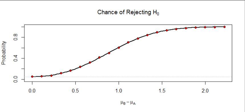
Generally, since you are considering the case $\mu_B\ge \mu_A,$ the first term in $(*)$ is less than $\alpha/2$ (and decreasing very rapidly as the difference of means increases) but the second term more than makes up for that, increasing quickly. Here is a plot of the chance of rejecting the null against the difference of means for sample size $n=10$ and test size $\alpha=0.05:4

The points are the actual rejection rates in 21 independent simulations of 10,000 pairs of datasets each: they fall along the curve, as one would hope.
This is the R code that produced the figure, written to parallel the analysis in this post.
#
# Theory: `f` is the power, `delta` is mu_B - mu_A, `n` is sample size.
#
f <- function(delta, n, alpha) {
  z <- qnorm(alpha/2)
  pnorm(z - sqrt(n/2)*delta) + pnorm(-z - sqrt(n/2)*delta, lower.tail=FALSE)
}
alpha <- 0.05
n <- 10
delta.max <- sqrt(2/n) * (3 - qnorm(alpha/2))
curve(f(x, n, alpha), 0, delta.max, ylim=0:1, lwd=2,
      main=expression(paste("Chance of Rejecting ", H[0])),
      xlab=expression(mu[B] - mu[A]),
      ylab="Probability")
abline(h=alpha, lty=3, col="Gray")
#
# Simulation: `delta` is mu_B-mu_A; `n` is sample size, `N` is # of replications
#
sim <- function(delta, n, N, alpha) {
  x <- matrix(rnorm(n*N), n)
  y <- matrix(rnorm(n*N, delta), n)
  z <- (colMeans(y) - colMeans(x)) * sqrt(n/2)   # The test statistic
  mean(abs(z) > -qnorm(alpha/2))                 # Empirical rate of rejection
}
delta <- seq(0, delta.max, length.out=21)
p <- sapply(delta, sim, n=n, N=1e4, alpha=alpha)
points(delta, p, pch=21, bg="Red")


