Fitting t-distribution in R: scaling parameter

Question

How do I fit the parameters of a t-distribution, i.e. the parameters corresponding to the 'mean' and 'standard deviation' of a normal distribution. I assume they are called 'mean' and 'scaling/degrees of freedom' for a t-distribution?

The following code often results in 'optimization failed' errors.

library(MASS)
fitdistr(x, "t")

Do I have to scale x first or convert into probabilities? How best to do that?

Answer 1

fitdistr uses maximum-likelihood and optimization techniques to find parameters of a given distribution. Sometimes, especially for t-distribution, as @user12719 noticed, the optimization in the form:

fitdistr(x, "t")

fails with an error.

In this case you should give optimizer a hand by providing starting point and lower bound to start searching for optimal parameters:

fitdistr(x, "t", start = list(m=mean(x),s=sd(x), df=3), lower=c(-1, 0.001,1))

Note, df=3 is your best guess at what an "optimal" df could be. After providing this additional info your error will be gone.

Couple of excerpts to help you better understand the inner mechanics of fitdistr:

For the Normal, log-Normal, geometric, exponential and Poisson distributions the closed-form MLEs (and exact standard errors) are used, and start should not be supplied.

...

For the following named distributions, reasonable starting values will be computed if start is omitted or only partially specified: "cauchy", "gamma", "logistic", "negative binomial" (parametrized by mu and size), "t" and "weibull". Note that these starting values may not be good enough if the fit is poor: in particular they are not resistant to outliers unless the fitted distribution is long-tailed.

Answer 2

MASS, the book (4th edition, page 110) advises against trying to estimate $\nu$, the degrees of freedom parameter in the $t$-distribution with maximum likelihood (with some literature references: Lange et al. (1989), "Robust statistical modeling Using the t distribution", JASA, 84, 408, and Fernandez & Steel (1999), "Multivariate Student-t regression models: Pitfalls and inference", Biometrika, 86, 1).

The reason is that the likelihood function for $\nu$ based on the t density function, may be unbounded and will in those cases not give a well defined maximum. Let us look at an artificial example where location and scale is known (as the standard $t$-distribution) and only the degrees of freedom is unknown. Below is some R code, simulating some data, defining the log-likelihood function and plotting it:

set.seed(1234)
n <- 10
x <- rt(n,  df=2.5)

make_loglik  <-  function(x)
    Vectorize( function(nu) sum(dt(x, df=nu,  log=TRUE)) )

loglik  <-  make_loglik(x)
plot(loglik,  from=1,  to=100,  main="loglikelihood function for df     parameter", xlab="degrees of freedom")
abline(v=2.5,  col="red2")

If you play around with this code, you can find some cases where there is a well-defined maximum, especially when the sample size $n$ is large. But is the maximum likelihood estimator then any good?

Let us try some simulations:

t_nu_mle  <-  function(x) {
    loglik  <-  make_loglik(x)
    res  <-  optimize(loglik, interval=c(0.01, 200), maximum=TRUE)$maximum
    res   
}

nus  <-  replicate(1000, {x <- rt(10, df=2.5)
    t_nu_mle(x) }, simplify=TRUE)

> mean(nus)
[1] 45.20767
> sd(nus)
[1] 78.77813

Showing the estimation is very unstable (looking at the histogram, a sizable portion of the estimated values is at the upper limit given to optimize of 200).

Repeating with a larger sample size:

nus  <-  replicate(1000, {x <- rt(50, df=2.5)
    t_nu_mle(x) }, simplify=TRUE)
> mean(nus)
[1] 4.342724
> sd(nus)
[1] 14.40137

which is much better, but the mean is still way above the true value of 2.5.

Then remember that this is a simplified version of the real problem where location and scale parameters also have to be estimated.

If the reason of using the $t$-distribution is to "robustify", then estimating $\nu$ from the data may well destroy the robustness.

Answer 3

In the help for fitdistr is this example:

fitdistr(x2, "t", df = 9)

indicating that you just need a value for df. But that assumes standardization.

For more control, they also show

mydt <- function(x, m, s, df) dt((x-m)/s, df)/s
fitdistr(x2, mydt, list(m = 0, s = 1), df = 9, lower = c(-Inf, 0))

where the parameters would be m = mean, s = standard deviation, df = degrees of freedom

Answer 4

You can use fitdistrplus library after extending the location and scaling parameters for the student t in base R according to this article on wikipedia. Below is sample code

library(fitdistrplus)
x<-rt(100,23)
dt_ls <- function(x, df=1, mu=0, sigma=1) 1/sigma * dt((x - mu)/sigma, df)
pt_ls <- function(q, df=1, mu=0, sigma=1)  pt((q - mu)/sigma, df)
qt_ls <- function(p, df=1, mu=0, sigma=1)  qt(p, df)*sigma + mu
rt_ls <- function(n, df=1, mu=0, sigma=1)  rt(n,df)*sigma + mu
fit.t<-fitdist(x, 't_ls', start =list(df=1,mu=mean(x),sigma=sd(x))) 
summary(fit.t)

Answer 5

The parameters of the t-distribution are referred to as the location, scale, and degrees of freedom $\nu$. The location can be estimated by the mean of the samples if $\nu > 1$; otherwise the mean is not defined. By not defined, this means that increasing the sample size will not converge to a particular value. The scale is a generalization of the standard-deviation. The scale $\sigma$ can be estimated from the standard-deviation of the samples if $\nu > 2$. $\sigma_{est} = E[(X-\mu)^2]^{1/2} sqrt[(\nu - 2)/\nu]$.

In addition to the established methods, new closed-formed estimates that achieve the maximum likelihood have been defined in two papers. In my paper "Use of the geometric mean as a statistic for the scale of the coupled Gaussian distribution" The Coupled Gaussian is equivalent to the Student's t but is expressed in terms of the shape or coupling, which is inverse to $\nu$. I showed a functional relationship between the scale, DoF and the geometric mean. Thus the function can be used to estimate either scale or DoF if the other is known.

In my paper "Independent Approximates enable closed-form estimation of heavy-tailed distributions" I showed that linear closed-form functions exist for estimating the location and scale parameters of the Student's t distribution. These functions are formed by selecting subsamples referred to as Independent Approximates (IAs). The IAs are formed by pairs, triplets, or n-tuples that are approximately equal. The IA-pairs are guaranteed to have a mean and can be used to estimate the location. The IA-triplets are guaranteed to have a finite second-moment and can be used to estimate the scale.

There is Mathematica code referenced in the IA paper. Perhaps someone would be interested in implementing the method in R.

Answer 6

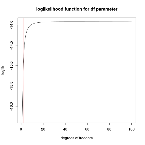
@SergeyBushmanov points out that sometimes you need to give maximum likelihood estimation a hand by providing appropriate starting point and lower/upper bounds for the optimization algorithm to find the MLE.

Another way to give the likelihood a hand is to augment it with a (weakly) informative prior and do Bayesian estimation. This approach is most applicable if we have domain information to help us formulate a useful prior.

I'll illustrate one Bayesian solution to the $t$ distribution fitting problem in the setting where @kjetilbhalvorsen demonstrates that the MLE approach fails: sample size $n = 10$, location $\mu = 0$, scale $\sigma = 1$ and degrees of freedom $\nu = 2.5$. I'll use the brms package to do the Bayesian model fitting and two different priors for the degrees of freedom $\nu$:

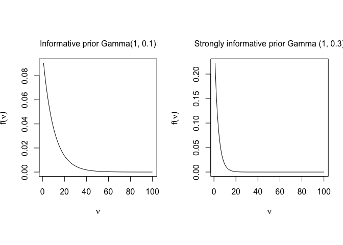
• strongly informative prior: $\nu \sim \operatorname{Gamma}(1, 0.3)$ and
• informative prior: $\nu \sim \operatorname{Gamma}(1, 0.1)$,

with the constraint $\nu > 1$ (otherwise the mean of the $t$ distribution is undefined.)

Both choices indicate there is high prior probability the degrees of freedom are less than 5: under the informative prior, $\operatorname{Pr}(\nu<5) = 0.33$ and under the strongly informative prior, $\operatorname{Pr}(\nu<5) = 0.7$. So both priors are quite "opinionated", which we would like to avoid in general. [The default brms prior on the degrees of freedom is $\operatorname{Gamma}(2, 0.1)$.] On the other hand, in general we would also probably collect more than $n = 10$ observations for a study where we know there is a lot of variability in the outcome.

And here is how to do Bayesian $t$ distribution fitting with brms::brm.

First we simulate a sample of size $n$ from $t(\mu=0,\sigma=1,\nu=2.5)$ where $\mu$ is the location, $\sigma$ is the scale and $\nu$ are the degrees of freedom.

n <- 10
mu <- 0
sigma <- 1
nu <- 2.5
x <- rt(n, nu) * sigma + mu

Then we fit an intercept-only $t$-family model.

fit.brm <- brm(
  x ~ 1,
  family = student,
  data = data.frame(x),
  prior = c(
    prior(student_t(3, 0, 2.5), class = "Intercept"),
    prior(student_t(3, 0, 2.5), class = "sigma"),
    prior(gamma(1, 0.3), class = "nu")
  )
)

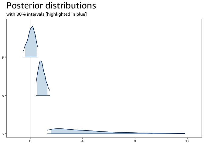
While the posterior distributions of the location $\mu$ and scale $\sigma$ are reasonably symmetric, the posterior of the degrees of freedom $\nu$ is very skewed. So I will use the posterior mode (rather than the posterior mean or the posterior median) to estimate the parameters.

round(
  apply(posterior, 2, mode), 3
)
#>     μ     σ     ν 
#> 0.161 0.785 2.164

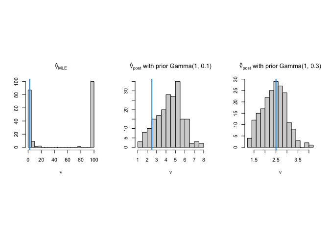
And finally, I repeat the three analyses (MLE, Bayesian with weakly informative prior, Bayesian with informative prior) 200 times. Each analysis estimates all three parameters (location $\mu$, scale $\sigma$ and degrees of freedom $\nu$) but below I plot histograms of the estimated degrees of freedom only. The true $\nu$ is 2.5.

Maximum likelihood estimation fails dramatically more than half of the time (100 is the upper bound for $\nu$ in the optimization). Bayesian estimation doesn't fail in any of the 200 simulations but the estimate is biased upwards unless the prior information indicates strongly that we expect a priori only a few degrees of freedom.