Variance estimate for Student's t-distribution with heavy tails

Question

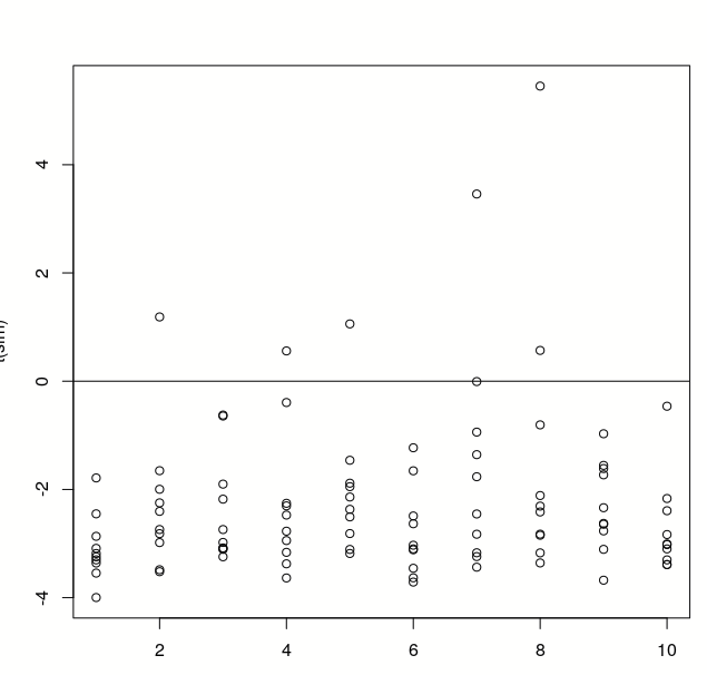
The variance of a Student's t random variable when the degrees of freedom $\nu$ is greater than $2$ is $\nu/(\nu-2)$. In R, when I try to estimate the variance using the usual estimator $$1/(n-1)\sum_{i=1}^n (x_i-\overline{x})^2$$, the estimates seem biased, when $\nu$ is close-ish to 2, like $\nu=2.2$. Here is my code and the output:

nu <- 2.2
sim <- sapply(round(seq(1e6, 5e6, len=10)), 
        function(n)replicate(10, var(rt(n, 
          nu)) - nu/(nu-2)))
matplot(t(sim), pch=1, col=1)
abline(h=0)

The estimated variance looks too small compared to the true variance. Is this

1. my sample sizes (up to 5 million) are still too small for the consistency to show for degrees of freedom this close to 2,

2. the sample variance estimator actually isn't consistent for these values of $\nu$,

3. something else?

Answer 1

As @whuber observes, the "usual" standard deviation estimate is highly variable when the underlying data is distributed $t$ with degrees of freedom just above 2.

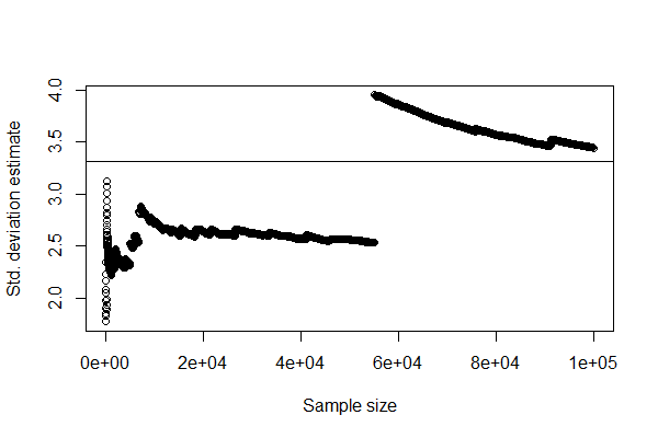
Consider the following experiment. We generate 100,000 samples from a $t(2.2)$ distribution, and calculate the sample standard deviation over successive sample sizes in steps of 10, e.g., x[1:10], x[1:20], ... x[1:100000]. We plot the results, which show the instability quite clearly:

df <- 2.2
x <- rt(100000, df)

sd_est <- rep(0, 10000)
for (i in seq_along(sd_est)) {
  sd_est[i] <- sd(x[1:(10*i)])
}

plot(sd_est ~ seq(1, length(x), 
       length.out=length(sd_est)),
     xlab = "Sample size", 
     ylab = "Std. deviation estimate")
abline(h=sqrt(df/(df-2)))  
# The true standard deviation

And the plot, with a horizontal line at the true value:

Even when we think we have a stable result, e.g., with sample sizes of 50,000, we can experience a big jump in our estimate with just one observation:

max(x)
[1] 712.4925
which.max(x)
[1] 55119 

And of course at no point in the trace are we particularly near the true value.

The solution is, as @whuber observes, to use a robust estimator. Note that estimating the parameters of the distribution using maximum likelihood, then calculating an estimate of the std. deviation from the estimated parameters, may also not be a good idea: see this answer to Fitting t-distribution in R: scaling parameter

Answer 2

Your example would be a good application of a new estimator for heavy-tailed distributions. I call the method Independent Approximates (IAs), since it utilizes a subsample of n-tuples that are approximately equal.

The method can be applied to estimate the location $\mu$, scale $\sigma$, and degree of freedom $\nu$. Since you are estimating the variance, I'll assume the scale is your primary interest.

To estimate the scale, assuming the location is known, one can use the triplet IAs. The triplet IAs are selected by partitioning the original samples into triplets and subselecting those triplets that are approximately equal, and retaining the median sample. The referenced paper provides further details. The triplet-IAs which are guaranteed to have a finite second moment for all $\nu$, and if $\nu > 2$ the variance of the second moment will be finite. For your example with $\nu=2.2$, the median triplet IA samples will have $\nu_{triplet} = 8.6$.

The estimate of the second moment of the triplets, $\mu_{triplet}^2$ can be used to estimate the scale of the original distribution using the following function $\mu = \sqrt{3 \mu_{triplet}^2}$.

See my paper Independent Approximates enable closed-form estimation of heavy-tailed distributions for further details and examples.

Answer 3

The distribution has a few large values. You don't see them when you plot only a hundred as in your example.

The example below shows more clearly that you get a mode that is unequal to zero but you do not necessarily have a mean unequal to zero.

set.seed(1)
nu <- 2.2
sim <- sapply(round(seq(1e4, 1e4, 
        len=10000)), function(n) 
         replicate(10, var(rt(n, nu)) - 
          nu/(nu-2)))

matplot(t(sim),pch=21,col=1, bg = 1, 
  cex = 0.5)
abline(h=0)

hist(sim, breaks = seq(min(sim-1), 
     max(sim+1), 0.25), xlim = c(-7,30))

mean(sim)
### the mean of this sample will equal 
### 2.297499, which is *above* zero